In my previous article I looked at what sort of advantage Julia has over Python/Numpy in terms of speed.

Although this is useful to know, it isn’t the whole story. It is also important to understand how they compare in terms of syntax, library availability / integration, flexibility, documentation, community support etc.

This article runs though an image classification deep learning problem from start to finish in both TensorFlow and Flux (Julia’s native TensorFlow equivalent). This should give a good overview of how the two languages compare in general usage, and hopefully help you get an insight into whether Julia is a potential option (or advantage) for you in this context.

I will also endeavour to highlight the advantages, and more importantly the gaps, or failings, that currently exist in the Julia ecosystem when compared to the tried and tested pairing of Python and TensorFlow.

Introduction #

I have deliberately chosen an image classification problem for this particular exploration, as it throws up some nice challenges in both data preparation, and for the deep learning frameworks themselves:

1. the images need to be loaded from disk (a ready prepared dataset such as MNIST will not be used), so loading and pre-processing methods and conventions will be explored
2. images are typically represented as 3D-matrices (height, width, colour channels), so careful attention to dimensional ordering will be required
3. to avoid over-fitting, image augmentation is typically required, allowing for an exploration into library availability and ease of use
4. images are inherently a ‘large’ data type in terms of space requirements, which forces an investigation into batching, RAM allocation and GPU usage

Note: Although code snippets will be made available throughout the article, Jupyter notebooks are available containing a full working end-to-end (image download through to model training) implementation of both the Julia and Python versions of the code. See the next section for links to the notebooks.

Incidentally, if this is the first time you have heard of Julia I recommend reading the “What is Julia?” section of my previous article to get a quick primer:

Is Julia Really Faster than Python and Numpy? The speed of C with the simplicity of Python Mike Clayton - Towards Data Science

Reference Notebooks #

This section gives details on the location of the notebooks, and also the requirements for the environment setup for online environments such as Colab and Deepnote.

The notebooks #

The raw notebooks can be found here for your local environment:

julia-python-image-classification null null - github.com

…or get kickstarted in either deepnote or colab.

Python Notebook:

Julia Notebook:

Environment Setup for Julia #

Deepnote #

As deepnote utilises docker instances, you can very easily setup a ‘local’ dockerfile to contain the install instructions for Julia. This means you don’t have to pollute the Jupyter notebook with install code, as you will have to do in Colab.

In the environment section select “Local ./Dockerfile”. This will open the actual Dockerfile where you should add the following:

FROM deepnote/python:3.10

RUN wget https://julialang-s3.julialang.org/bin/linux/x64/1.8/julia-1.8.3-linux-x86_64.tar.gz && \
    tar -xvzf julia-1.8.3-linux-x86_64.tar.gz && \
    mv julia-1.8.3 /usr/lib/ && \
    ln -s /usr/lib/julia-1.8.3/bin/julia /usr/bin/julia && \
    rm julia-1.8.3-linux-x86_64.tar.gz && \
    julia  -e "using Pkg;pkg\"add IJulia\""

ENV DEFAULT_KERNEL_NAME "julia-1.8"

You can update the above to the latest Julia version from this page, but at the time of writing 1.8.3 is the latest version.

Colab #

For colab all the download and install code will have to be included in the notebook itself, as well as refreshing the page once the install code has run.

Fortunately, Aurélien Geron has made available on his GitHub a starter notebook for Julia in colab, which is probably the best way to get started.

Note: if you use the “Open in Colab” button above (or the Julia notebook ending in “colab” from the repository I linked) I have already included this starter code in the Julia notebook.

The Data #

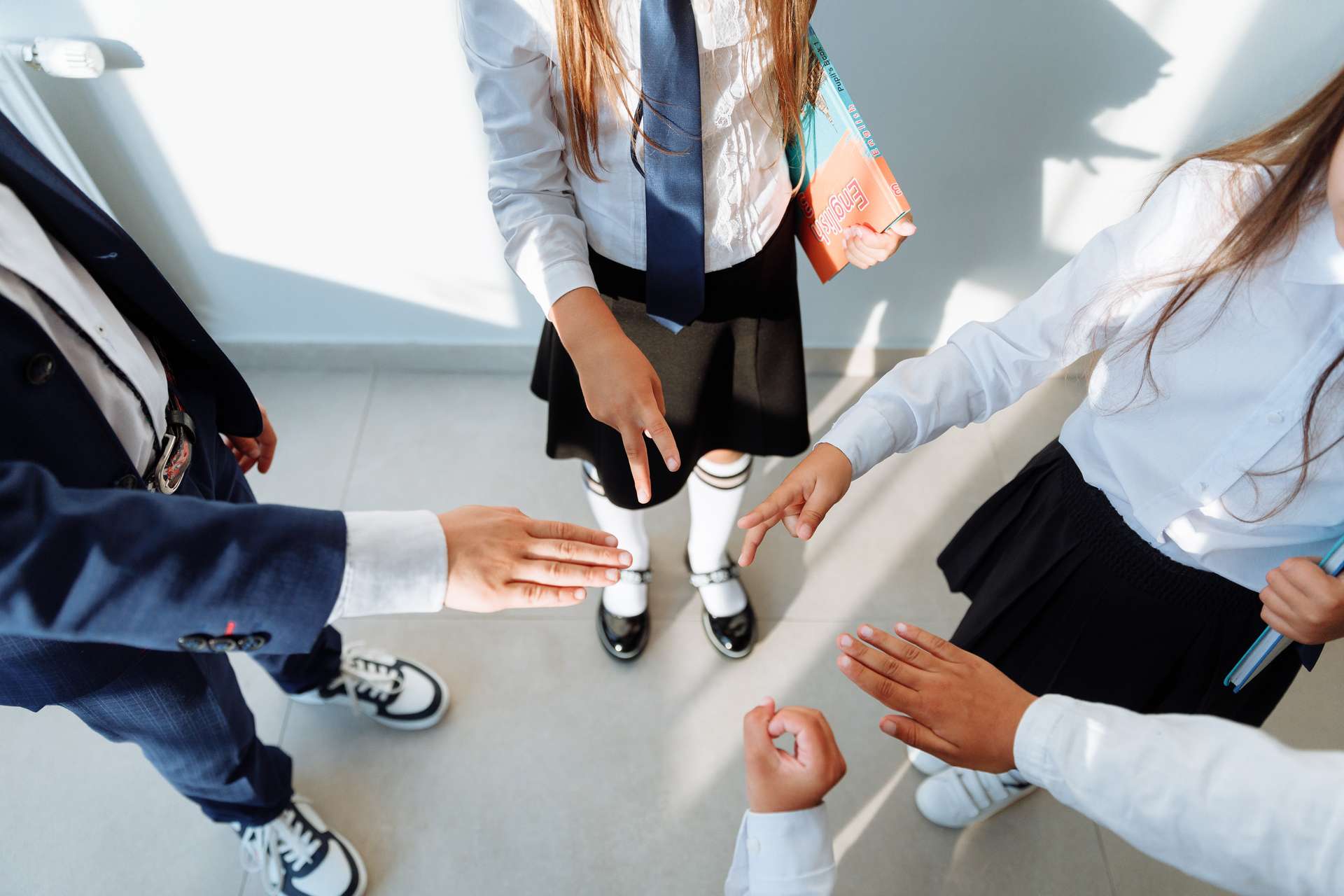
The data^[1] utilised in this article is a set of images which depict the three possible combinations of hand position used in the game rock-paper-scissors.

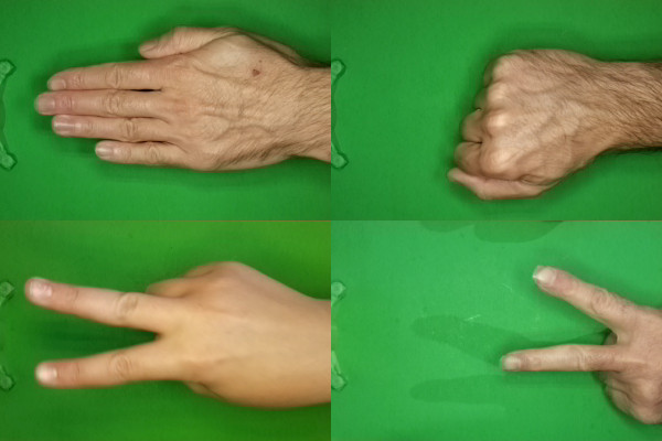
Four examples from the three different categories of the dataset. Composite image by Author.

Each image is of type PNG, and of dimensions 300(W) pixels x 200(H) pixels, in full colour.

The original dataset contains 2188 images in total, but for this article a smaller selection has been used, which comprises of precisely 200 images for each of the three categories (600 images in total). This is mainly to ensure that the notebooks can be run with relative ease, and that the dataset is balanced.

The smaller dataset that was used in this article is available here:

rock_paper_scissors null null - github.com

The Plan #

There are two separate notebooks. One written in Python using the TensorFlow deep learning framework, and a second that is written in Julia and utilises the Flux deep learning framework.

Both notebooks use exactly the same raw data, and will go through the same steps to finally end up with a trained model at the end.

Although it is not possible to match the methodology exactly between the two notebooks (as you might expect), I have tried to keep them as close as possible.

A general outline #

Each notebook covers the following steps:

1. Download the image data from a remote location and extract into local storage
2. Load the images from a local folder structure ready for processing
3. Review image data, and view sample images
4. Split the data into train / validation sets
5. Augment the training images to avoid over-fitting
6. Prepare the images for the model (scaling etc.)
7. Batch data
8. Create model and associated parameters
9. Train model (should be able to use the CPU or GPU)

Comparison — Packages #

Photo by Leone Venter on Unsplash

The comparison sections that follow will explore some of the differences (good or bad) that Julia has with the Python implementation. It will generally be broken down as per the bullet points in the previous section.

Package installation #

To start with, a quick note on package installation and usage.

The two languages follow a similar pattern:

1. make sure the package is installed in your environment
2. ‘import’ the package into your code to use it

The only real difference is that Julia can either install packages in the ‘environment’ before running code, or the packages can be installed from within the code (as is done in the Julia notebook for this article):

“Pkg” in Julia is the equivalent of “pip” in Python, and can also be accessed from Julia’s command line interface.

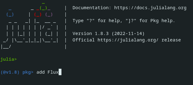
An example of adding a package using the command line. Screenshot by author

Package usage #

In terms of being able to access the installed packages from within the code, you would typically use the keyword “using” rather than “import”, as used in Python:

Julia does also have an “import” keyword too. For more details on the difference please take a look at the documentation. In most general use cases “using” is more appropriate.

Note: in this article I have deliberately used the full path, including the module names, when referencing a method from a module. This is not necessary, it just makes it clearer which package the methods are being referenced from. For example these two are equivalent and valid:

using Random

Random.shuffle(my_array) # Full path

shuffle(my_array) # Without package name

Comparison — Download and Extraction #

Photo by Miguel Á. Padriñán on Pexels

The image data is provided remotely as a zip file. The zip file contains a folder for each of the three categories, and each folder has 200 images contained within.

First step, download and extract the image files. This is relatively easy in both languages, and with the available libraries, probably more intuitive in Julia. The Python implementation:

What the Julia implementation could look like:

using InfoZIP

download("https://github.com/thetestspecimen/notebooks/raw/main/datasets/rock_paper_scissors/rock_paper_scissors.zip","./rock_paper_scissors.zip")

root_folder = "rps"
isdir("./$root_folder") || mkdir("./$root_folder")

InfoZIP.unzip("./rock_paper_scissors.zip", "./$root_folder")

You may notice that I said what it it could look like. If you look at the notebooks you will see that in Julia I have actually used a custom function to do the unzipping, rather than utilising the InfoZIP package as detailed above.

The reason for this is that I couldn’t get the InfoZIP package to install in all of the environments I used, so I thought it would be unfair to include it.

Is this a fault of the package? I suspect not. I think this is likely due to the fact that the online environments (colab and deepnote) are not primarily geared towards Julia, and sometimes that can cause problems. InfoZIP installs and works fine locally.

Is this a fault of the package? I suspect not.

I should also note here that to use the “Plots” library (which is the equivalent of something like matplotlib) in colab when utilising a GPU instance will result in failure to install!

This may seem relatively trivial, but it is a direct illustration of the potential problems you can run into when dealing with a new-ish language. Furthermore, you are less likely to find a solution to the problem online as the community is smaller.

It is still worth pointing out that when working locally on my computer I had no such issues with either package, and I would hope that with time online environments such as colab and deepnote may be a bit more Julia friendly out of the box.

Comparison — Handling images #

Photo by Ivan Shimko on Unsplash

Now the images are in the local environment, it is possible to take a look at how we can load and interact with them.

Python:

Julia:

In the previous section things were relatively similar. Now things start to diverge…

This simple example of loading an image highlights some stark differences between Python and Julia, although that might not be immediately obvious from two similar looking code blocks.

Zero indexing vs one indexing #

Probably one of the major differences between the languages in general, is the fact that Julia uses indexing for arrays and matrices starting from 1 rather than 0.

Python — the first element of “random_image”:

img = mpimg.imread(target_folder + "/" + random_image[0])

Julia — the first element of the shape of “image_channels”:

println("Colour channels: ", size(img_channels)[1])

I can see how this could be a contentious difference. It all comes down to preference in reality, but putting any personal preferences aside, 1-indexing makes a lot more sense mathematically.

It is also worth remembering the field of work this language is aimed at (i.e. more mathematical / statistics based professionals who are programming, rather than pure programmers / software engineers).

Regardless of your stance, something to be very aware of, especially if you are thinking of porting a project over to Julia from Python.

How images are loaded and represented numerically #

When images are loaded using python and “imread” they are loaded into a numpy array with the shape (height, width, RGB colour channels) as float32 numbers. Pretty simple.

In Julia, images are loaded as:

Type: Matrix{RGB{N0f8}}

Not so clear…so let’s explore this a little.

In JuliaImages, by default all images are displayed assuming that 0 means “black” and 1 means “white” or “saturated” (the latter applying to channels of an RGB image).

Perhaps surprisingly, this 0-to-1 convention applies even when the intensities are encoded using only 8-bits per color channel. JuliaImages uses a special type, N0f8, that interprets an 8-bit "integer" as if it had been scaled by 1/255, thus encoding values from 0 to 1 in 256 steps.

-Juliaimages.org

Turns out this strange convention used by Julia is actually really helpful for machine / deep learning.

One of the things you regularly have to do when dealing with images in Python is to scale the values by 1/255, so that all the values fall between 0 and 1. This is not necessary with Julia, as the scaling is automatically done by the “N0f8” type used for images natively!

Unfortunately, you will not see the comparison in this article as the images are type PNG, and imread in Python returns the array as float values between 0 and 1 anyway (incidentally the only format it does that for).

Photo by Michael Maasen on Unsplash

However, if you were to load in a JPG file in Python, you would receive integer values between 0 and 255 as the output from imread, and have to scale them later in your pre-processing pipeline.

Apart from the auto scaling, it is also worth noting how the image is actually stored. Julia uses a concept of representing each pixel as a type of object, so if we look at the output type and shape:

Type: Matrix{RGB{N0f8}}
Shape: (200, 300)

It is literally stated as a 200x300 matrix. What about the three colour channels? We would expect 200x300x3, right?

Well, Julia views each of the items in the 200x300 matrix as a ‘pixel’, which in this case has three values representing Red, Green and Blue (RGB), as indicated in the type ‘RGB{N0f8}’. I suppose it would be like a matrix of objects, the object being defined as having three variables.

However, there is reason behind the madness:

This design choice facilitates generic code that can handle both grayscale and color images without needing to introduce extra loops or checks for a color dimension. It also provides more rational support for 3d grayscale images–which might happen to have size 3 along the third dimension–and consequently helps unify the “computer vision” and “biomedical image processing” communities.

-Juliaimages.org

Some real thought went into these decisions it would seem.

However, you cannot feed an image in this format into a neural network, not even Flux, so it will need to be split out into a ‘proper’ 3D matrix at a later stage. Which as it turns out is very easy indeed, as you will see.

Comparison — Data preparation pipeline #

Photo by JJ Ying on Unsplash

This is definitely one of the areas where, in terms of pure ease of use Python and TensorFlow blow Julia out of the water.

The Python implementation #

I can more or less load all my images into a batched optimised dataset ready to throw into a deep learning model in essentially four lines of code:

Training image augmentation is taken care of just as easily with a model layer:

The Julia implementation #

To achieve the same thing in Julia requires quite a bit more code. Let’s load the images and split them into train and validation sets:

I should note that in reality, you could lose the “load and scale” and “shuffle” sections of this method and deal with it in a more terse form later, so it isn’t as bad as it looks. I mainly left those sections in as a reference.

One useful difference between Python and Julia is that you can define types if you want, but it is not absolutely necessary. A good example is the type of “Tuple{Int,Int}” specified for the “image_size” in the function above. This ensures whole numbers are always passed, without having to do any specific checking within the function itself.

Augmentation pipeline #

Image augmentation is very simple just like TensorFlow thanks to the Augmentor package, you can also add the image resizing here using the “Resize” layer (a more terse form as alluded to earlier):

You should also note that Augmentor (using a wrapper of Julia Images) has the ability to change the ‘RGB{N0f8}’ type to a 3D matrix of type float32 ready for passing into the deep learning model:

I want to break down the three steps above as I think it is important to understand what exactly they do, as I can see it is potentially quite confusing:

1. SplitChannels — takes an input of Matrix{RGB{N0f8}} with shape 160 (height) x 160 (width) and converts it to 3 (colour channels) × 160 (height) × 160 (width) with type Array{N0f8}. It is worth noting here that the colour channels become the first dimension, not the last like in python/numpy.
2. PermuteDims — just rearranges the shape of the array. In our case we change the dimensions of the output to 160 (width) x 160 (height) x 3 (colour channels). Note: the order of height and width have also been switched.
3. ConvertEltype — changes N0f8 into float32.

You may be wondering why the dimensions need to be switched about so much. The reason for this is due to the requirement of the input shape into a Conv layer in Flux at a later stage. I will go into more detail once we have completed batching, as it one of my main gripes with the whole process…

Applying the augmentation #

Now we have an interesting situation. I need to apply the augmentation pipelines to the images. No problem! Due to the excellent augmentbatch!() function provided by the Augmentor package.

Except no matter how hard I tried I couldn’t get it to work with the data. Constant errors (forgot to note down exactly what while I was frantically trying to sort out a solution, but there were similar problems in various forums).

There is always the possibility that this is my fault, I kind of hope it is!

As a workaround, I used a loop using the ‘non-batched’ method augment. I also one-hot encoded the labels at the same time using the OneHotArrays package:

I think this goes a long way to illustrate that there are some areas of the Julia ecosystem that may give you a few implementation headaches. You may not always find a solution online either, as the community is smaller.

However, one of the major advantages of Julia is that if you have to resort to things like a for loop to navigate a problem, or just to implement a bit of a bespoke requirement, you can be fairly sure that the code you write will be optimised and quick. Not something you can rely on every time with Python.

Some example augmented images from the train pipeline:

Batching the data #

Batching in Julia is TensorFlow level easy. There are multiple ways of going about this in Julia. In this case Flux’s built in DataLoader will be used:

Nothing much to note about the method. Does exactly what it says on the tin. (This is the alternative place you can shuffle the data as I alluded to earlier.)

We are ready to pass the data to the model, but first a slight detour…

Confusing input shapes #

Photo by Torsten Dederichs on Unsplash

I now want to come back to the input shape for the model. You can see in the last code block of the previous section that the dataset has shape:

Data: 160(width) x 160(height) x 3(colour channels) x 32(batchsize)
Labels: 3(labels) x 32(batchsize)

In TensorFlow the input shape would be:

Data: 32(batchsize) x 160(height) x 160(width) x 3(colour channels)
Labels: 32(batchsize) x 3(labels)

From the Julia documentation:

Image data should be stored in WHCN order (width, height, channels, batch). In other words, a 100×100 RGB image would be a 100×100×3×1 array, and a batch of 50 would be a 100×100×3×50 array.

-fluxml.ai

I have no idea why this convention has been chosen, especially the switching of height and width.

Frankly, there is nothing to complain about, it is just a convention. In fact, if previous experience is anything to go by I would suspect some very well thought out optimisation is the cause.

I have come across some slightly odd changes in definition compared to other languages, only to find out there is a very real reason for it (as you would hope).

As a concrete (and relevant) example, take Julia’s Images package.

The reason we use CHW (i.e., channel-height-width) order instead of HWC is that this provides a memory friendly indexing mechanism for Array. By default, in Julia the first index is also the fastest (i.e., has adjacent storage in memory). For more details, please refer to the performance tip: Access arrays in memory order, along columns

-juliaimages.org

Extra confusion #

This brings up one of the main gripes I have.

I can accept that it is a different language, so there is potentially a good reason to have a new convention. However, during the course of loading images and getting them ready for plugging into a deep learning model in Flux, I have had to morph the input shape all over the place:

1. Images are loaded in: Matrix{RGB{N0f8}} (height x width)
2. Split channels: {N0f8} (channels x height x width)
3. Move channels AND switch height and width: {N0f8} (width x height x channels)
4. Convert to float32
5. Batchsize (as last element): {float32} (width x height x channels x batchsize)

As apparently (channels x height x width) is optimal for images, and that is how native Julia loads them in. Could it not be:

(channels x height x width x batchsize)?

Might save a lot of potential confusion.

I genuinely hope that someone can point out that I have stupidly overlooked something (really I do). Mainly because I have been very impressed with the attention to detail and thought that has gone into designing this language.

OK. Enough moaning. Back to the project.

Comparison — The model #

Photo by DS stories on Pexels

Model definition in Julia is very similar to the Sequential method of TensorFlow. It is just called Chain instead.

Note: I will mostly cease to include the TensorFlow code in the article at this point just to keep it readable, but both notebooks are complete and easy to reference if you need to.

Main differences:

1. You must explicitly load both the model (and data) onto the GPU if you want to use it
2. You must specify the input and output channels explicitly (input=>output) — I believe there are shape inference macros that can help with this, but we won’t get into that here

All in all very intuitive to use. It also forces you to have a proper understanding of how the data moves and reshapes through the model. A good practise if you ask me.

There is nothing more dangerous that a black box system, and no thinking. We all do it of course as sometimes we just want the answer quickly, but it can lead to some hard to trace and confusing outcomes.

There is nothing more dangerous than a black box system, and no thinking. We all do it…

Calculation device specification #

In the code for the notebook you can see where I have explicitly defined which device (CPU or GPU) should be used for calculation by using the variable “calc_device”.

Changing the “calc_device” variable to gpu will use the gpu. Change it to cpu to use only the cpu. You can of course replace all the “calc_device” variables with gpu or cpu directly, and it will work in exactly the same way.

Comparison — Loss, Accuracy and Optimiser #

Image by 3D Animation Production Company from Pixabay

Again, very similar to TensorFlow:

A couple of things of note:

logitcrossentropy #

You may have noted that the model has no softmax layer (if not take a quick look).

This is mathematically equivalent to crossentropy(softmax(ŷ), y), but is more numerically stable than using functions crossentropy and softmax separately.

-fluxml.ai

onecold #

The opposite of onehot. Excellent name, not sure why someone hasn’t thought of that before.

One line function definition #

If you are new to Julia it is also worth pointing out that the loss and accuracy functions are actually proper function definitions in one line. i.e. the same as this:

function loss(X, y)
  return Flux.Losses.logitcrossentropy(model(X), y)
end

One of many great features of the Julia language.

(Note: you could actually omit the return keyword in the above. Another way of shortening a function.)

Comparison — Training #

Photo by Victor Freitas on Unsplash

Training can be as complicated or simple as you like in Julia. There is genuinely a lot of flexibility available, I haven’t even touched the surface in what I’m about to show you.

If you want to keep it really simple there is what I would call the equivalent to “model.fit” in TensorFlow:

for epoch in 1:10
    Flux.train!(loss, Flux.params(model), train_batches, opt)
end

That’s right, basically a for loop. You can also add a callback parameter to do things like print loss or accuracy (which is not done automatically like TensorFlow), or early stopping etc.

However, using the above method can cause problems when dealing with large amounts of data (like images), as it requires loading all of the train data into memory (either locally or on the GPU).

The following function therefore allows the batches to be loaded onto the GPU (or memory for a CPU run) batch by batch. It also prints the training loss and accuracy (an average over all batches), and the validation loss on the whole validation dataset.

Note: If the validation set is quite large you could also calculate the validation loss/accuracy on a batch by batch basis to save memory.

In reality, it is two for loops: one for the epochs and an internal loop for the batches.

The lines of note are:

x, y = device(batch_data), device(batch_labels)
gradients = Flux.gradient(() -> loss(x, y), Flux.params(model))
Flux.Optimise.update!(optimiser, Flux.params(model), gradients)

This is the loading of a batch of data onto the device (cpu or gpu), and running the data through the model.

All the rest of the code is statistics collection and printing.

More involved than TensorFlow, but nothing extreme.

…and we are done. An interesting journey.

Summary (and TL;DR) #

Photo by Ann H on Pexels

At the beginning of the article I stated that apart from speed there are other important metrics when it comes to deciding if a language is worth the investment compared to what you already use. I specifically named:

1. syntax
2. flexibility
3. library availability / integration
4. documentation
5. community support

Having been over a whole project I thought it might be an idea to summarise some of the findings. Just bear in mind that this is based on my impressions while generating the code for this article, and is only my opinion.

Syntax #

Coming from Python I think that the syntax is similar enough that it is relatively easy to pick up, and I would suggest that in quite a few circumstances it is even more ‘high level’ and easy to use than Python.

Let’s get the contentious one out of the way first. Yes, Julia uses 1-indexed arrays rather than 0-indexed arrays. I personally prefer this, but I suspect there will be plenty who won’t. There are also more subtle differences such as array slicing being inclusive of the last element, unlike Python. Just be a little careful!

But there is plenty of good stuff…

For example when using functions you don’t need a colon or return keyword. You can even make a succinct one liner without losing the codes meaning:

# this returns the value of calculation, no return keyword needed

function my_func(x , y)
      x * y + 2
end

# you can shorten this even further

my_func(x, y) = x * y + 2

Notice the use of “end” in the standard function expression. This is used as indentation doesn’t matter in Julia, which in my opinion is a vast improvement. The spaces vs tabs saga will not apply to Julia.

The common if-else type statements can also be utilised in very terse and clear one line statements:

# ternary - if a is less than b print(a) otherwise print(b)

(a < b) ? print(a) : print(b)

# only need to do something if the condition is met (or not met)? 
# use short circuit evaluation.

# if a is less than b print(a+b), otherwise do nothing

(a < b) && print(a+b)

# if a is less than b do nothing, otherwise print(a+b)

(a < b) || print(a+b) 

I’m likely just scratching the surface here, but already I am impressed.

Flexibility #

I think flexibility is something that Julia really excels at.

As I have already mentioned, you can write code that is terse and to the point just like Python, but there are also additional features should you need, or want, to utilise them.

The first and foremost is probably the option to use types, something not possible in Python. Although inferred types sound like a great idea, they do have various downsides, such as making code harder to read and follow, and introducing hard to trace bugs.

flexibility to specify types when it makes the most sense is an excellent ability

Having the flexibility to specify types when it makes the most sense is an excellent ability that Julia has. I’m glad it isn’t forced across the board though.

Julia is also aimed at scientific and mathematical communities. Utilising unicode characters in your code, is therefore quite a useful feature. Not something I will likely use, but as I come from a mathematical / engineering background I can appreciate the inclusion.

Library availability / consistency #

This is a bit of a mixed bag.

Photo by Iñaki del Olmo on Unsplash

This article has utilised quite a few packages. From some larger packages such as Flux and Images, right down to more bespoke packages such as OneHotArrays and Augmentor.

On the whole I would say they don’t, on average, approach the level of sophistication, integration, and ease of use that you can find in Python / TensorFlow. It takes a little bit more effort do the same thing, and you are likely to find more problems, and hit more inconsistencies. I am not surprised by this, at the end of the day it is a less mature ecosystem.

For example the ability to batch and optimise your data with a simple one line interface is a really nice feature of TensorFlow. The fact you don’t have to write extra code to print training and validation loss / accuracy is also very useful.

However, I think Julia’s library ecosystem has enough variation and sophistication to genuinely do more than enough. The packages on the whole play nicely together too. I don’t think it is even close to a deal breaker.

To summarise my main issues I encountered with the packages in this article:

1. I couldn’t get the package InfoZIP to install consistently across all environments
2. I couldn’t get the !augmentbatch() function to work for the data in this article at all, which would have been useful
3. For some reason there is a slightly muddled approach to how the shape of an image is defined between JuliaImages and Flux, which leads to quite a lot of messing about with re-shaping matrices. It isn’t hard, it just seems unnecessary.

Documentation #

Documentation for the core language is a pretty complete and reliable source. The only thing I would suggest is that the examples given for some methods could be a bit more detailed and varied. A minor quibble, otherwise excellent stuff.

Moving beyond the core language, and the detail and availability of the documentation can vary.

I’m impressed with the larger packages, which I suppose would be almost core packages anyway. In terms of this article, that would be JuliaImages and Flux. I would say they are pretty comprehensive, and I particularly like the effort that goes into emphasising why things are done a certain way:

The reason we use CHW (i.e., channel-height-width) order instead of HWC is that this provides a memory friendly indexing mechanisim for Array. By default, in Julia the first index is also the fastest (i.e., has adjacent storage in memory).

-juliaimages.org

As the packages get smaller, the documenation is generally there, but a bit terse. ZipFile is a good example of this.

Although, typically packages are open source and hosted on Github, and contributions are usually always welcome. As stated by JuliaImages:

Please help improve this documentation–if something confuses you, chances are you’re not alone. It’s easy to do as you read along: just click on the “Edit on GitHub” link above, and then edit the files directly in your browser. Your changes will be vetted by developers before becoming permanent, so don’t worry about whether you might say something wrong.

-juliaimages.org

Community #

The community is exactly what I expected it to be, lively and enthusiastic, but significantly smaller than Python’s / TensorFlow’s. If you need answers to queries, especially more bespoke queries, you may need to dig a little deeper than you usually would into the likes of Google and StackOverflow.

This will obviously change with adoption, but fortunately the documentation is pretty good.

Conclusion #

All things considered I think Julia is a great language to actually use.

The creators of the language were trying to take the best parts of the languages they loved to use, and combine them into a sort of super language, which they called Julia.

In my opinion they have done an extremely good job. The syntax is genuinely easy to use and understand, but can also incorporate advanced and slightly more obscure elements — it is a very flexible language.

It is also genuinely fast.

Image by Wokandapix from Pixabay

Yes, there may be a slight learning curve to switch from the language you are using at the moment, but again, I don’t think it will be as severe as you might think. To help you out, Julia’s documentation includes a nice point by point comparison for major languages:

Noteworthy Differences from other Languages · The Julia Language Although MATLAB users may find Julia’s syntax familiar, Julia is not a MATLAB clone. There are major syntactic and functional differences. The following are some noteworthy differences that may trip up Julia users accustomed to MATLAB: null - julialang.org

The only downsides I see are due to the fact that it is, even after 10 year of existence, relatively new compared to it’s competitors. This has a direct impact on the quality and quantity of documentation and learning resources. Which appears to have a bigger impact on adoption than most people would like to admit. Money also helps, as always…but I don’t have the data to comment on that situation.

Being the best product or solution does not guarantee success and broad acceptance. That is just not how the real world works.

…but after getting to know how Julia works (even on a basic level) I do hope more people see the potential and jump onboard.

References #

[1] Julien de la Bruère-Terreault, Rock-Paper-Scissors Images (2018), Kaggle, License: CC BY-SA 4.0

🙏🙏🙏

Since you've made it this far, sharing this article on your favorite social media network would be highly appreciated. For feedback, please ping me on Twitter.

...or if you want fuel my next article, you could always:

Published 02 Dec 2022