The purpose of this article is to look into whether the use of the Continuous Wavelet Transform (CWT) is beneficial as a preprocessing technique before utilising a neural network to predict a human gesture classification problem.
There will be no heavy mathematics, with the focus being on the implementation, and results. Where necessary some explanation will be provided as to why certain parameters are used.
Why use the CWT? #
One of the main challenges with machine learning is feeding in data that is going to be easy for the model to interpret and learn from, without losing any important information from the original data. If you can achieve this, it allows for simpler lightweight models, and reduces the chances of, for example, over-fitting to noise or other anomalies in your raw data.
The CWT can potentially help you achieve this.
The basics #
The CWT is a signal processing technique similar to the Fourier Transform, in that it lets you extract and separate out frequency information from a timeseries. Where it differs from the Fourier Transform is that it can also retain the time domain information as well (i.e. it can display the frequency data and where it occurred along the timeseries).
The output for a single 2D input time series (x: time, y: amplitude) is therefore a 3D output matrix (x: time, y: frequency, z: amplitude). This means the output of a CWT can be rendered as a pictogram (i.e. visualised in a 2D image rather than a line).
Where is the advantage? #
We have turned the original signal into a picture, which is great for humans, as it is more interpretable for us. However, we are going to feed this into a neural network, so if it contains the same information as the original signal why bother?
Turns out you have a few dials to play with when tuning the transform that will differentiate your CWT output from the original signal.
Choosing your wavelet #
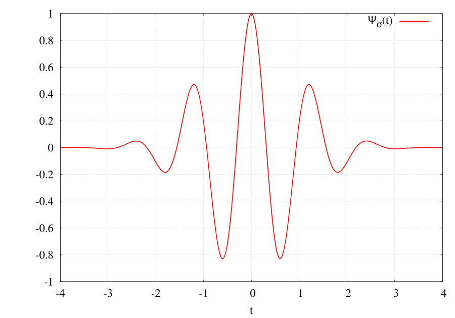
There are predefined wavelets that you can use against the signal. Each wavelet is different in terms of shape and characteristics, you should pick a wavelet shape that fits well with the characteristics of the signal you are trying to process. I won't go further into this selection process here, but if unsure the Morlet wavelet is a good starting point, and what we will use throughout this article.
The wavelet is basically convolved (multiplied) with the time series at each timestep, moving across the signal. This is done at varying 'scales', so scale 1 will be for high frequencies (i.e. the wavelet is narrow and picks up higher frequencies in the signal). As you increase the scale the wavelet is stretched horizontally, and therefore a better match to lower frequencies. This process is repeated for a variety of scales which allows the extraction of frequency information from the signal.
Setting the scale #
As mentioned in the previous section you can stretch the signal using a parameter called 'scale'. This is equivalent of targeting specific frequencies within the signal.
You can literally specify a range of scales to be processed, so this gives you the flexibility to, for example, filter out high frequency noise from the signal. Or very specifically target a certain frequency range.
Use as an exploratory tool #
As mentioned earlier you can make visualisations from the CWT, so one approach might be to visually review a random selection of data to help determine where the most appropriate 'scale' range is, and fine tune the scale to that range before passing to the neural network.
Complex wavelets #
Some of the wavelet transforms are complex (i.e. the wavelets extend into the complex domain). Ultimately, this means that you can extract phase information from a signal, if this is of use for your analysis. However, it is worth noting that this is an additional layer of information that may be useful for a neural network. We will utilise complex wavelets (in a very superficial way) in this article.
Why not use the Discrete Wavelet Transform (DWT)? #
You may have heard of the Discrete Wavelet Transform (DWT), and wonder why we don't use that?
The truth is they are very similar (both being wavelet transforms), however to get into the differences at any meaningful level requires a dive into mathematics, which is not what this article is for.
Very simply the DWT also breaks down the signal into frequency components. However, each 'level' of detail (like the scales in the CWT) extracted from the original time series results in a halving of the samples (i.e. the signal gets shorter). This is more efficient computationally than the CWT, but not ideal for our purposes here. You can't produce an image for example.
What the DWT is very useful for is filtering. As an example, if you want to filter noise from your signal the DWT is an excellent choice, but that is beyond the remit of this article.
The data #
Direct quote from the data source:
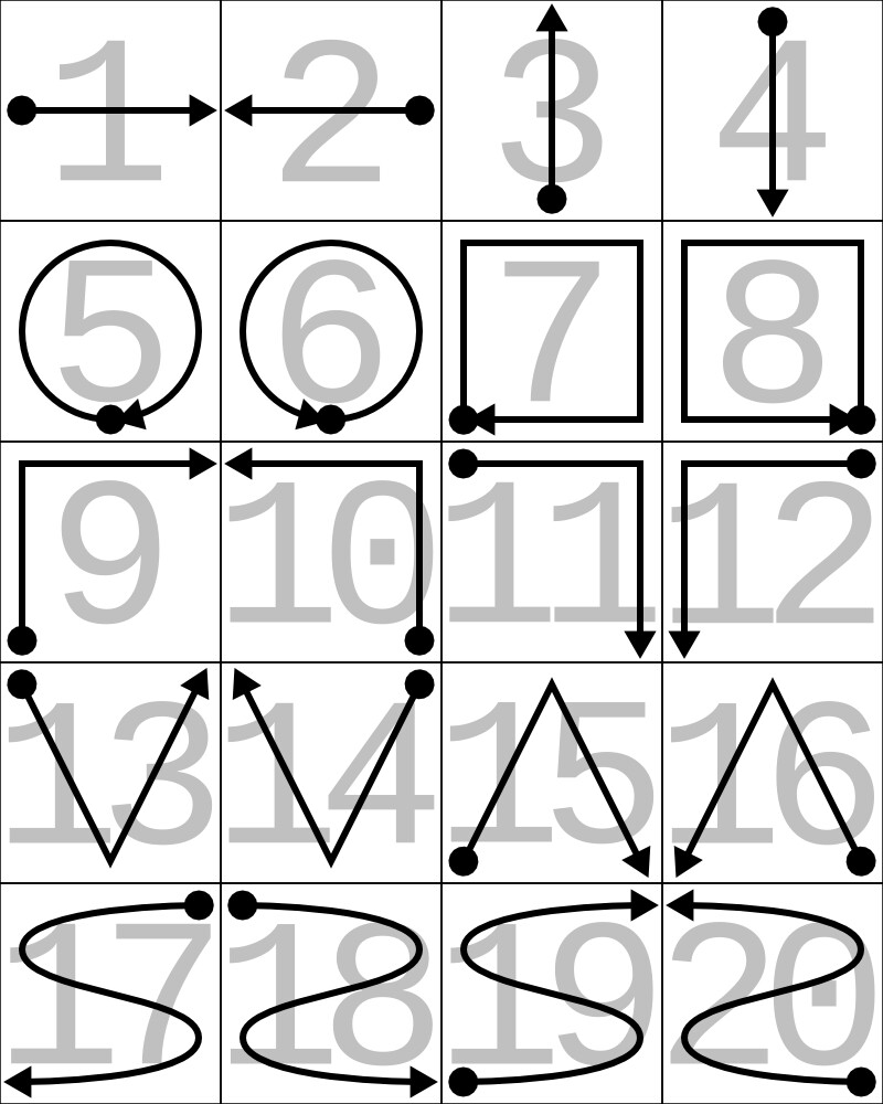
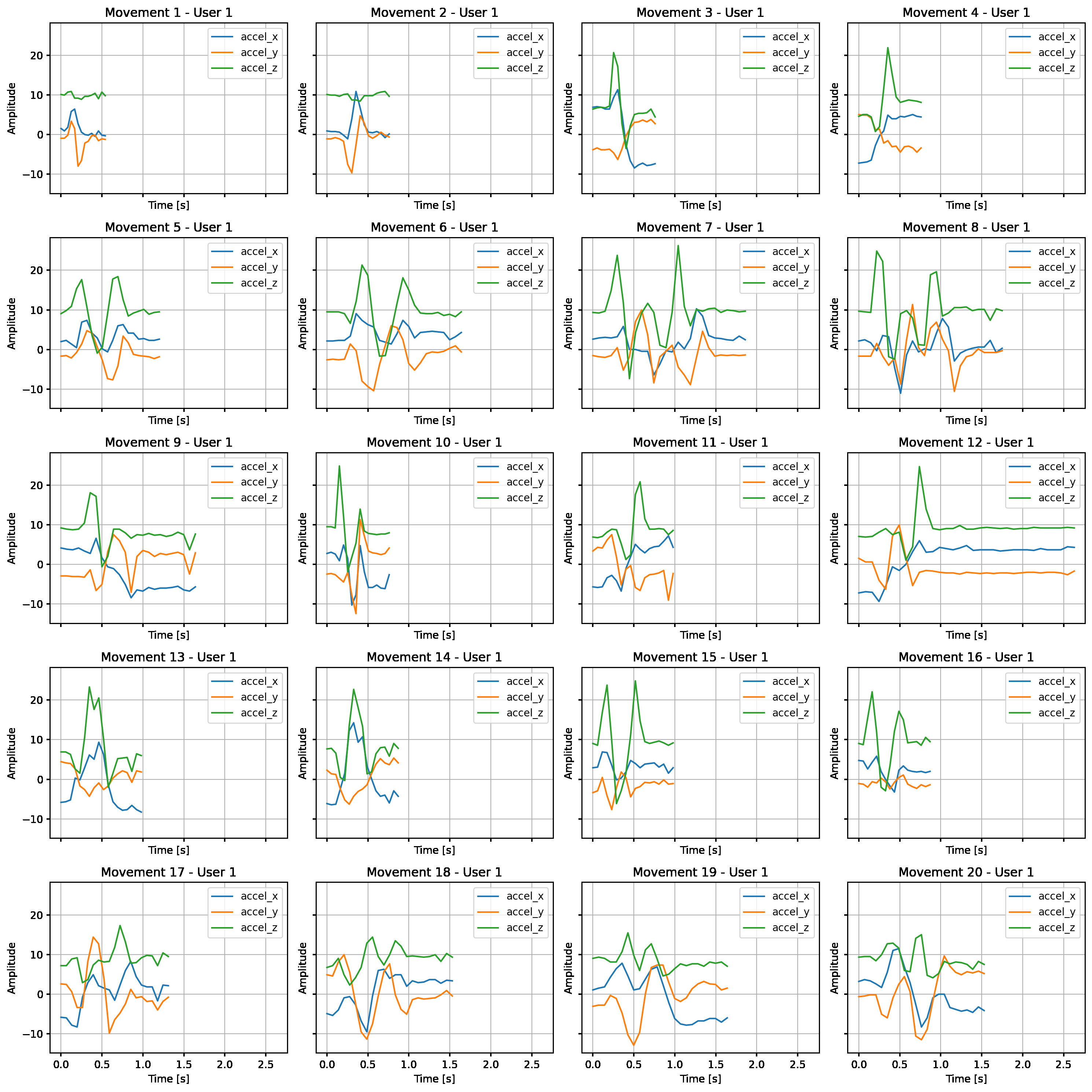
Eight different users performed twenty repetitions of twenty different gestures, for a total of 3200 sequences. Each sequence contains acceleration data from the 3-axis accelerometer of a first generation Sony SmartWatch™, as well as timestamps from the different clock sources available on an Android device. The smartwatch was worn on the user's right wrist. The gestures have been manually segmented by the users performing them by tapping the smartwatch screen at the beginning and at the end of every repetition.
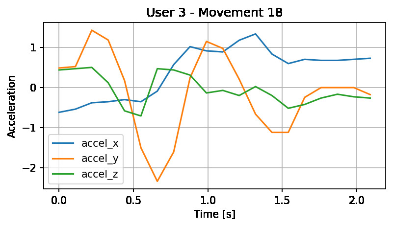
An example of each of the movements performed by the participants and their associated labels can be seen in the image below:
The plan #
This is the overall plan of how the data will be prepared and compared.
If you wish to look in detail at the code used to produce the results that follow, please feel free to reference the jupyter notebook, which is available on my github here:
Data split #
Initially, I will use 7 out of the 8 people as training and validation, and the 8th person as a holdout test set.
The 7 people will be completely randomised and then split 85%-15% (train-validation). The final outcome of the models being judged on the holdout test 'person'.
This should result in:
- training timeseries --> 2380 sequences
- validation timeseries --> 420 sequences
- testing timeseries --> 400 sequences
Total timeseries: 3200
Models #
The models that will be created are as follows:
- Model 1 - A CNN model (Conv1D) used as a baseline on the raw timeseries data - this is the benchmark
- Model 2 - A CNN model (Conv2D) utilising a CWT on the timeseries before input into the model
- Model 3 - A CNN model (Conv2D) utilising a complex CWT on the timeseries before input into the model
All the above models will use the same parameters and number/type of layers to keep them as comparable as possible.
Comparison #
Stage 1 #
A single run of the model to get an idea of accuracy and see where the model is failing (or succeeding) to generalise.
(Users 1 to 7 as train/validation, User 8 as holdout test).
Stage 2 #
Ten repeat runs to get a more accurate average accuracy, which removes any variation due to numerical randomness / initialisation parameters.
(Users 1 to 7 as train/validation, User 8 as holdout test).
Stage 3 #
For Model 1 and either Model 2 or 3 (depending which performs best), a cross validation of users will be performed.
Essentially, each individial user (1 to 8) will be used as the hold out test set in a completely independent set of tests. Each set of tests will be repeated 10 times (like Stage 2) to get an average accuracy.
This will give a good indication as to how the models perform for each individual, ultimately giving a better indication as to how the model will likely perform with a completely new user in the future.
Preprocessing the data #
Exploration #
In an initial exploration of the data the following points were discovered:
- the data is sampled at around 9Hz (0.11s per sample)
- the timeseries samples are all of different lengths (longest 51 sample (5.61s), average of 20 samples (2.2s))
- the total amount of timeseries is not 3200 it is actually 3251, with some users having more samples than others (although still a very even split, not highly skewed to one user or another)
- the accelerometer data is close to normally distributed for the purposes of scaling
- accelerometer in the z direction looks to have a more significant mean offset from zero than the other two components (possibly gravity?)
Preprocessing #
One of the initial problems with the dataset is that the timeseries are all of different lengths. This means we need to pad the sequences to length of the longest sequence (assuming we don't want to truncate the data).
We will take two different approaches here. The first will be for the raw timeseries data and the second for the data intended for the CWT.
As the data crosses zero we will use a large padding value (-9999.0) on the timeseries input data, and then use a masking layer to mask these values in the model. As the CWT is a pre-processor before the model, we cannot feed exaggerated padding values like this into the CWT, as it will heavily skew the data. A zero pad will therefore be used on the data that will be fed into the CWT.
To ensure that the zero pad will not skew the data too much SciKitLearn's StandardScaler will be used to scale the data to zero mean and unit variance before applying the pad (we have already confirmed the data is relatively normally distributed so this should be appropriate). For consistency, and the benefits scaling generally provides for neural networks anyway, this scaling will also be applied to the raw time series data used in the reference model (Model 1).
All models will also include a scaling layer to scale the input data between the values of 1 and -1 before hitting the neural network. The scaling value used will be based on the highest absolute value across all accelerometers after standard scaling (rather than each individually) to retain relative magnitude between the sensors.
Note: the data used to fit StandardScaler consisted of the whole dataset. Only the training dataset should really be used for this otherwise you leak information about the validation and test sets, which are meant to be independent. In this particular case it is not a big deal, as we are just exploring, but if you have to present reliable bulletproof figures, please do not do this.
Picking scales for the CWT #
One of the items that first needs to be considered before jumping into preprocessing the data with a CWT is what scales you wish to compute the continuous wavelet transform over, as this will decide how well the signal is represented in the output.
The scales are arbitrary, but a sensible selection can be made by translating the scales into associated frequencies. Scales can be 'translated' into frequencies if the sample rate of the data is known. Basically, a small scale (1 for example) is related to a higher frequency, and a larger scale to a lower frequency. This is basically due to the increase in scale 'stretching' the wavelet, and hence being a better match to 'longer' signals (i.e. lower frequencies).
In our case the sample rate of the data is approximately 9Hz (0.11 seconds, sample to sample). This is not a particularly high sample rate, so we need to retain as much of the data as possible.
Unfortunately, the CWT is subject to the Nyquist frequency, so in theory any frequency above 4.5Hz will experience aliasing, which is not ideal as it will polute the signal.
At the other end of the scale:
Our longest signal is 51 timesteps long which is 5.61s (which is about 0.18Hz). The average signal is 20 timesteps long which is 2.20s (which is about 0.45Hz)
This gives a good starting point for picking our scales. To keep the output small, as we are not using particularly deep neural networks, we will limit the lower frequency to about half the maximum, so ~0.36Hz and try to get as close to 4.5Hz as we can. This should give us a nice range to work with.
Here is the code which shows the result of the above. The output is an array of frequencies hitting the range we discussed above:
# Standard Morlet Wavelet frequencies at double the sampling frequency
dt = 0.11  # ~9 Hz sampling
input_scales = np.arange(2,22, dtype='float32')
input_scales = np.insert(input_scales,0,1.64)
frequencies = pywt.scale2frequency('morl', input_scales) / dt
frequencies

array([4.5038805 , 3.6931818 , 2.4621212 , 1.8465909 , 1.4772726 ,
       1.2310606 , 1.0551947 , 0.92329544, 0.8207071 , 0.7386363 ,
       0.67148757, 0.6155303 , 0.5681818 , 0.52759737, 0.49242425,
       0.46164772, 0.434492  , 0.41035354, 0.38875598, 0.36931816,
       0.35173163], dtype=float32)

# Complex Morlet Wavelet frequencies at double the sampling frequency
input_scales_comp = np.arange(2,27, dtype='float32')
frequencies = pywt.scale2frequency('cmor1.5-1.0', input_scales_comp) / dt
frequencies

array([4.5454545 , 3.0303032 , 2.2727273 , 1.8181819 , 1.5151516 ,
       1.2987014 , 1.1363636 , 1.0101011 , 0.90909094, 0.8264463 ,
       0.7575758 , 0.6993007 , 0.6493507 , 0.6060606 , 0.5681818 ,
       0.53475934, 0.50505054, 0.4784689 , 0.45454547, 0.43290043,
       0.41322315, 0.39525694, 0.3787879 , 0.36363634, 0.34965035],
      dtype=float32)
So from the above we can see that the appropriate scales to hit our intended frequency ranges for the data will be:
Morlet: 1.64 to 21
Complex morlet: 2 to 26
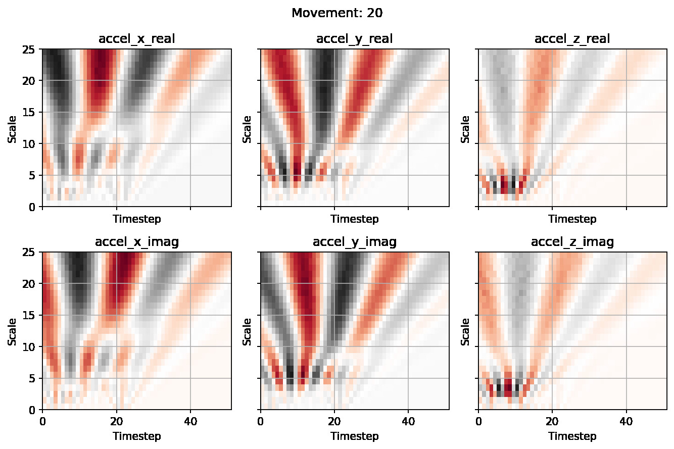
Note: In the example above there are six graphs as the complex wavelet has both imaginary and real parts. The normal CWT will produce only three graphs, as there are no imaginary parts.
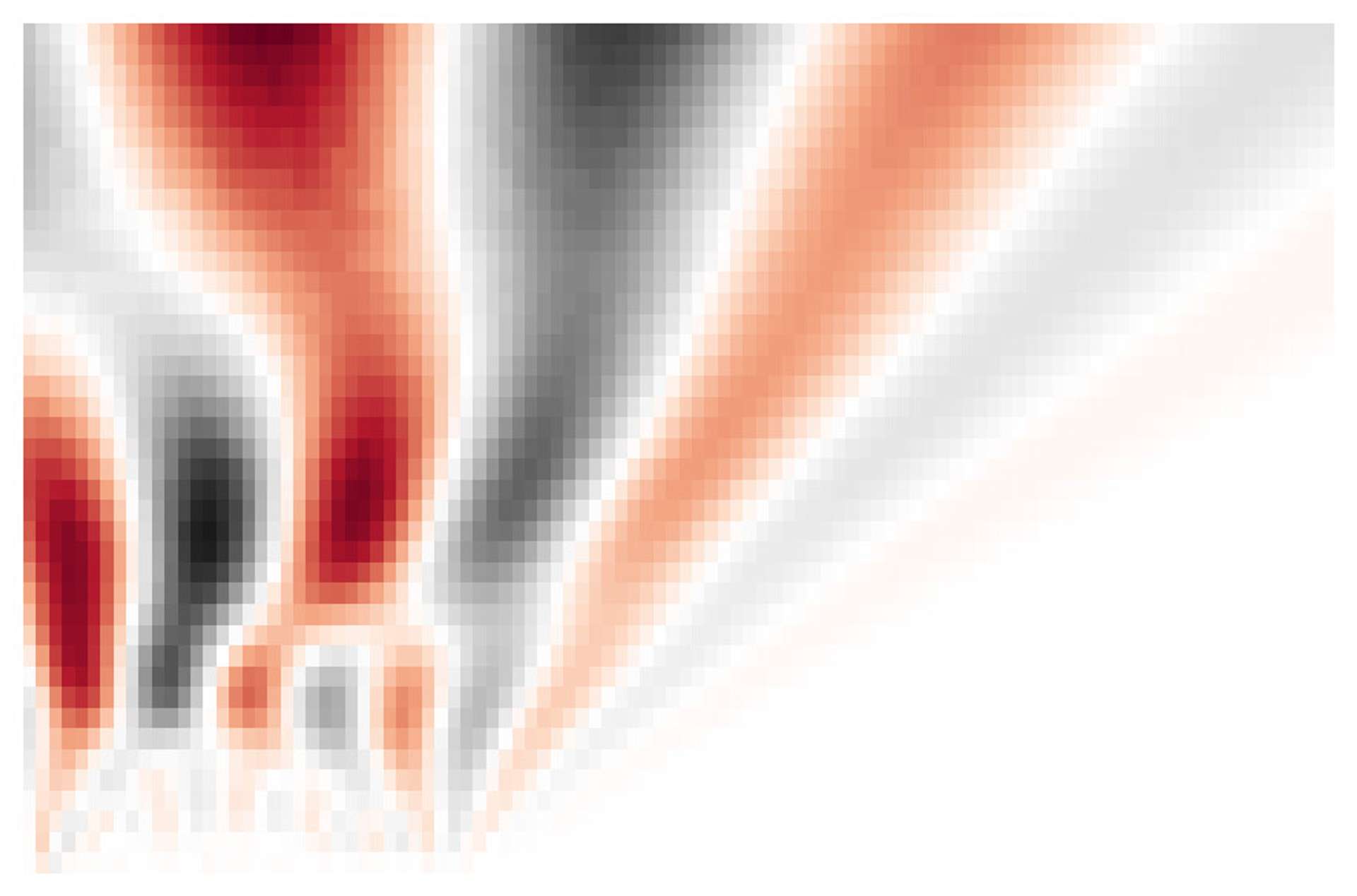
What do the graphs show? #
The graphs above are printed in grey and red fading to white at the centre value (roughly zero in this case). I have left a scale bar off as it is mostly irrelevant due to the data being scaled. So when you see dark red or dark grey, those are high energy areas (peaks or troughs). This is where most of the information resides in our signal.
You can immediately see both in terms of time and scale (or frequency) where in the signal has the most information. This could help you further tune the scales to focus on a particular area of interest, should you want to experiment further.
The models #
The models were constructed to be as close as possible, and simple. I have included dropout and pooling layers in the model to reduce overfitting since the data is limited and not particularly complicated.
# Model 1 - for raw timeseries data
if model_number == 1:
model = Sequential([
Input(shape=input_shape),
Masking(mask_value=-9999.0),
Rescaling(scaling_value),
Conv1D(filters=64,
kernel_size=4,
strides=1,
padding='valid',
kernel_initializer='glorot_uniform',
activation='relu'),
MaxPooling1D(),
Dropout(0.2),
Conv1D(filters=32,
kernel_size=1,
strides=1,
padding='valid',
kernel_initializer='glorot_uniform',
activation='relu'),
MaxPooling1D(),
Flatten(),
Dense(64, activation='relu'),
Dropout(0.2),
Dense(20,activation='softmax')
],name='Conv1D_Model_1')
# Model 2 - for CWT images
# (Model 3 (for the complex CWT) is the same as this, but has been cut for brevity)
elif model_number == 2:
model = Sequential([
Input(shape=input_shape),
Rescaling(scaling_value),
Conv2D(filters=64,
kernel_size=4,
strides=1,
padding='valid',
kernel_initializer='glorot_uniform',
activation='relu'),
MaxPooling2D(),
Dropout(0.2),
Conv2D(filters=32,
kernel_size=1,
strides=1,
padding='valid',
kernel_initializer='glorot_uniform',
activation='relu'),
MaxPooling2D(),
Flatten(),
Dense(64, activation='relu'),
Dropout(0.2),
Dense(20,activation='softmax')
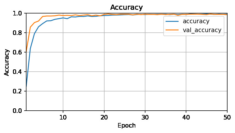
],name='CWT_Model_2')The models are all compiled with the Adam optimiser and run for 50 epochs each. At the end of the 50 epochs the best weights are restored based on val_loss.
Learning rates were tuned once for each model prior to the main runs:
- Model 1 - 0.005
- Model 2 - 0.001
- Model 3 - 0.001
On the main runs a scheduler also halved the learning rate every 20 epochs to help the model converge.
The results #
All models managed an accuracy and val_accuracy of 99%. Game over? Not really...
What that means is that our models have all learnt really well (or over-fit). Remember, our test and validation set is a random mixture of 7 users, but the hold out test set is a completely different person that doesn't exist at all in training or validation sets. So for the trained models on the initial run on the holdout test set (User 8):
| Model | Accuracy | F1-Score |
|---|---|---|
| 1 (Raw time-series) | 0.88 | 0.88 |
| 2 (CWT) | 0.93 | 0.92 |
| 3 (Complex CWT) | 0.96 | 0.96 |
For an initial run that result looks pretty impressive! We still need to repeat the runs 10 times like we said at the start to remove any initialisation randomness and see how stable the outputs are, but it is looking promising.
What might be interesting is to see where the models are making mistakes...
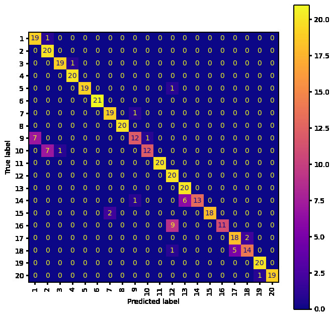
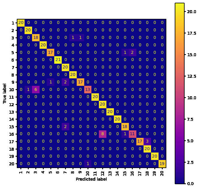
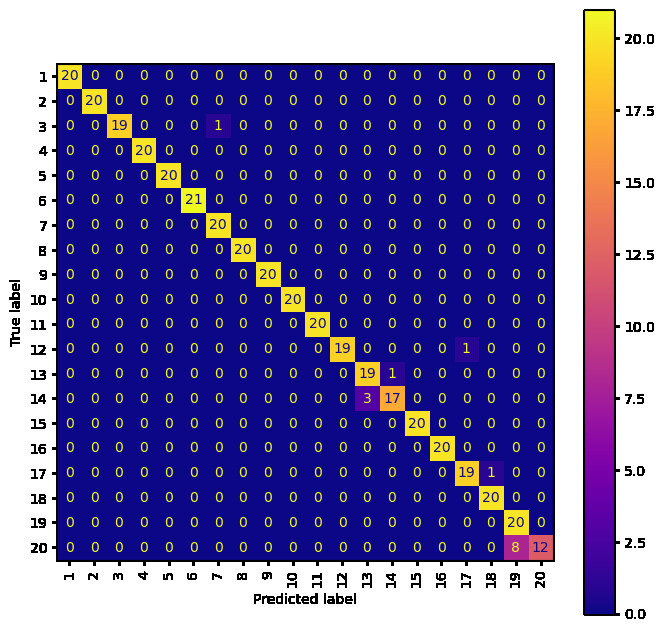
As you can see by comparing the movements to Model 1 and 3, the movements that the models get wrong make a lot of sense (i.e. they are similar movements). The worst mismatched predicted labels are:
- Model 1 - 16 confused with 12
- Model 2 - 16 confused with 12
- Model 3 - 20 confused with 19
Interestingly, although Model 3 on the whole does a better job, Model 1 manages to almost perfectly classify label 20 whereas Model 3 struggles with this particular label. It shows that the information is there, but Model 3 fails to capture it, or it has been removed by the transform. To further solidify this point, Model 2 also performs well for label 20, so the CWT is capable of capturing the correct information, but some fine tuning of scales is probably required.
Solidifying the numbers #
To get a more solid grasp on the how the models perform the tests were repeated 10 times and the result averaged:
| Model | Accuracy |
|---|---|
| 1 (Raw timeseries) | 0.859 |
| 2 (CWT) | 0.945 |
| 3 (Complex CWT) | 0.952 |
A box plot as another visual aid as to the results distribution:
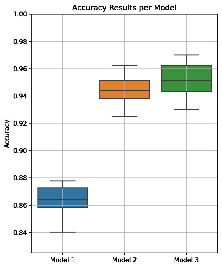
The result of this is that there is a fairly significant advantage to using a CWT on this data (at least under the parameters used in this article). It is also noted that, although the difference is small, it may be beneficial to consider a complex wavelet transform to try and extract as much data as possible out of the time series before processing.
The definitive check - cross validation #
In the previous sections we have explored the benefit of using the continuous wavelet transform in a neural network. So far the hold out test set has been user 8. However, we have no idea whether this user is a good representation of the general population, or a fairly unique individual.
A cross validation across all users will therefore be run (i.e. each user will be the hold out test set for it's own set of train/val/test runs). This should give a much more reliable indication of the performance that has been achieved, especially considering the small size of the dataset.
To avoid any bias due to randomness, we will also repeat each test 10 times and take an average, as we have done previously.
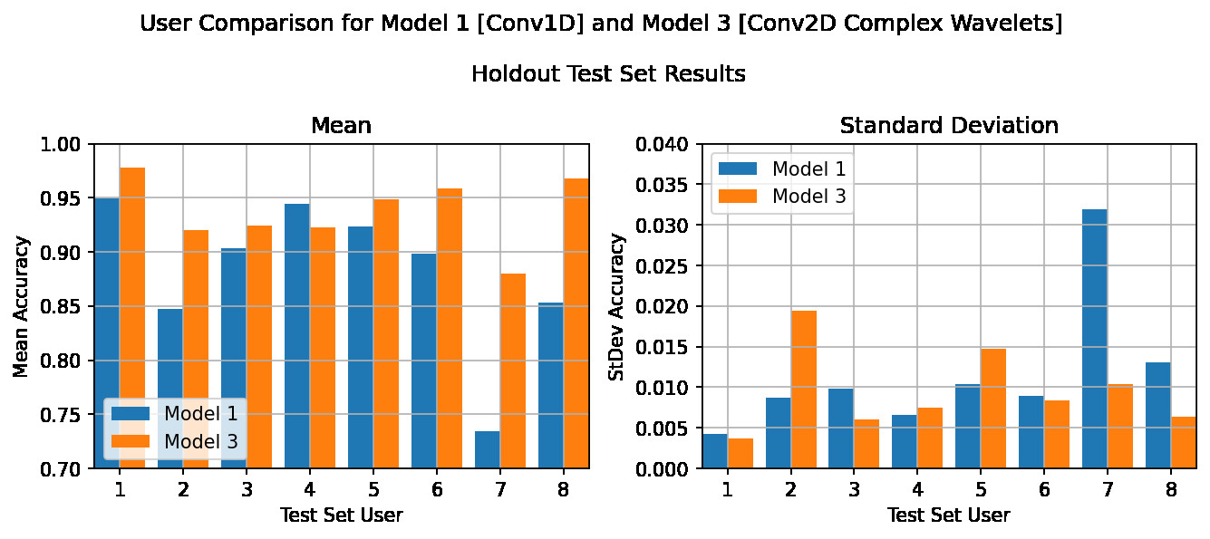
It seems the hold out user really does matter! Although there are a wide variation of results, depending on the user, almost across the board the CWT transform outperforms the normal time series model (from 2% to 15% improvement). The exception, as you can see, is User 4, where the CWT is beaten on average by the normal model. Although it should be noted that there is only a 2% difference, and Model 3 managed a quite respectful 92% accuracy in this case.
Note: the standard deviation graph presented is calculated across the 10 repeat runs for each user, and represents how consistent the model is across the 10 repeat runs.
Further to the above, it should be noted that the validation results across all tests and all users was very high (97%+).
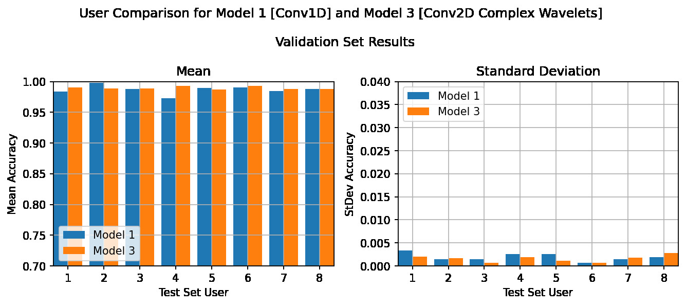
This indicates that although the models were able to learn the data provided to them equally well, the CWT model was able to both, pick out more relevant features, and generalise better than than the normal time series model.
Conclusion #
In this particular case I think we can conclude that the CWT should definitely be considered as a tool in the arsenal of machine learning practitioners. It will not be suitable for every case, perhaps because of the additional overhead of processing that is required. However, it is a flexible tool that can be moulded to suit your specific data, and potentially improve model bias and accuracy.
This article has only really touched the surface, as no in depth tuning of parameters has been performed. Items like the complex parameters of the complex Morlet wavelet were fixed throughout this experiment, and plenty of experimentation of a suitable range of scales could be conducted, so there is plenty of scope for further investigation in to the CWTs use in machine learning.
References #
From the authors of the dataset:
- G. Costante, L. Porzi, O. Lanz, P. Valigi, E. Ricci, Personalizing a Smartwatch-based Gesture Interface With Transfer Learning, 22nd European Signal Processing Conference, EUSIPCO 2014
- L. Porzi and S. Messelodi and C.M. Modena and E. Ricci: A Smart Watch-based Gesture Recognition System for Assisting People with Visual Impairments. ACM International Workshop on Interactive Multimedia on Mobile and Portable Devices - IMMPD, Barcelona, Spain, 2013
Other references and articles of interest:
Introduction to redundancy rules: the continuous wavelet transform comes of age
Multiple Time Series Classification by Using Continuous Wavelet Transformation
🙏🙏🙏
Since you've made it this far, sharing this article on your favorite social media network would be highly appreciated. For feedback, please ping me on Twitter.
...or if you want fuel my next article, you could always:

Published