In the real world you will often find that data follows a certain probability distribution. Whether it is a Gaussian (or normal) distribution, Weibull distribution, Poisson distribution, exponential distribution etc., will depend on the specific data.

Being aware of which distribution describes your data, or likely best describes your data, allows you to take advantage of that fact, and improve your inference and/or predictions.

This article will look at how leveraging knowledge of an underlying probability distribution of a dataset can improve the fit of a bog standard K-Means clustering model, and even allow for automatic selection of the number of appropriate clusters, directly from the underlying data.

Introduction #

A lot of the headline grabbing machine / deep learning techniques tend to involve supervised machine / deep learning i.e. the data has been labelled, and the models are given the correct answers to learn from. The trained model is then applied to future data to make predictions.

This is all very useful, but the reality is that data is constantly being produced by businesses and people around the world, and the majority of it is not labelled. It is actually quite expensive and time consuming to label data in the vast majority of cases. This is where unsupervised learning comes in.

…data is constantly being produced by businesses and people around the world, and the majority of it is not labelled.

Finding the best way to infer meaning from unlabelled data is a very important pursuit for many businesses. It allows the unearthing of potentially unknown, or less obvious, trends or groupings. It is then possible to assign resources, target specific groups of customers, or just instigate additional research and development.

Further to this, a large majority of the time, the data involves people or natural processes in one form or other. Natural processes, and the behaviour of people are, more often than not, captured and described well by a Gaussian distribution.

With this in mind, this article will take a look into how a Gaussian distribution, in the form of both a Gaussian Mixture Model (GMM) and a Bayesian Gaussian Mixture Model (BGMM), can be utilised to improve the clustering accuracy of a dataset that represents ‘natural processes’ encountered in real world datasets.

As a comparison and base for judgement, the ubiquitous K-Means clustering algorithm will be used.

The Plan? #

Photo by Christina Morillo from Pexels

This article will cover quite a lot of ground, and also incorporate examples from a comprehensive Jupyter notebook.

This section should give you some guidance on what is covered and where to skip to should you need access to specific information.

1. Initially the article will cover the “what” and “why” questions in regard to the use of Gaussian Mixture Models in general.
2. As there are two readily available implementations of Gaussian Mixture Models within the scikit-learn library, a discussion of the key differences between a plain Gaussian Mixture Model and Bayesian Gaussian Mixture Model will follow.
3. The article will then dive into using Gaussian Mixture Models to cluster a real world multi-featured dataset. All examples will be implemented using K-Means, a plain Gaussian Mixture Model and a Bayesian Gaussian Mixture Model.
4. There will then be two additional sections primarily focused on clearer visualisation of the algorithms. Complexity of the data will be reduced by a) using a two component principle component analysis (PCA) and b) analysing only two features from the dataset

Note: the dataset chosen is in fact labelled. This has been done deliberately so that the performance of the clustering can be compared to the 100% correct and known primary clustering.

The Explanations #

Photo by Polina Zimmerman from Pexels

Here we cover the “what” and “why” type questions before getting stuck into the data to see it all in action.

Before we get started, it is worth noting that there will be no discussion of what a Gaussian / Normal distribution is, or even what K-Means clustering is. There are plenty of great resources out there, and there just isn’t the space to cover it in this article. Therefore, a basic understanding of those concepts is assumed from this point on.

Note: the phrases “Gaussian distribution” and “Normal distribution” mean one and the same thing, and will be used interchangeably throughout this article.

What is a Gaussian Mixture Model? #

In simple terms, the algorithm assumes that the data you provide it can be approximated with an unspecified mixture of different Gaussian distributions.

The algorithm will try to extract and separate this mixture of Gaussian distributions and pass them back to you as separate clusters.

That’s it really.

So in essence, it is like K-Means clustering, but it has the added advantage of being able to apply additional statistical constraints on the data. This gives more flexibility to the shape of the clusters it can capture. In addition, it allows closely spaced, or slightly conjoined, clusters to be separated more precisely, as the algorithm has access to the statistical probabilities generated by the assumed Gaussian distributions.

In a visual sense, if the analysis is restricted to two or three dimensions, the K-Means algorithm pins down cluster centres and applies a ‘circular’ or ‘spherical’ distribution around those centres.

However, if the underlying data is Gaussian it is perfectly possible, and even expected, that the distribution will be elongated to some extent due to the tails of a Gaussian distribution. This would be the equivalent of an ‘ellipse’ or ‘ellipsoid’ in terms of shape. These elongated ‘ellipse’ or ‘ellipsoid’ type shapes are something K-Means cannot model accurately, but the Gaussian Mixture Models can.

On the other side of the coin, if you pass the Gaussian Mixture Models data that is definitely nowhere near Gaussian, the algorithm will still assume it is Gaussian. You will therefore likely end up with, at best, something that is no better than K-Means.

Side note: the Gaussian Mixture Model and Bayesian Gaussian Mixture Model can use the K-Means clustering algorithm to generate some of the initial parameters of the model (it is in fact the default setting in scikit-learn).

Which begs the question…

What type of data could Gaussian Mixture Models be used for? #

Natural processes are usually a good place to start. The reason for this is mainly due to the Central Limit Theorem (CLT):

In probability theory, the central limit theorem (CLT) establishes that, in many situations, when independent random variables are summed up, their properly normalized sum tends toward a normal distribution even if the original variables themselves are not normally distributed.

-wikipedia.org

In very simple terms, what this essentially means with natural processes is that although the particular variable (a humans height for example) is caused by many factors that may, or may not, be normally distributed (diet, lifestyle, environment, genes etc.) the normalised sum of those parts (the human height) will be (approximately) normally distributed. That is why we tend to see natural processes appearing to be normally distributed so regularly.

Photo by Ivan Samkov from Pexels

As such, there are a surprisingly large amount of real world instances where it is necessary to deal with Gaussian distributions, making Gaussian Mixture Models a very useful tool if it used in the appropriate setting:

• Customer behaviour — this could be in terms of purchases made, amounts spent, attention span, churn etc.
• Human characteristics — height, weight, shoe size, IQ (or educational performance) etc.
• Natural phenomena — recognition of patterns / groups in the medical field (cancers, diseases, genes etc.) or other scientific fields

There are obviously many other examples, and other situations where a Gaussian distribution may arise for other reasons.

There may of course be cases where you cannot discern the underlying structure of the data, and this will of course warrant investigation, but is also one of the reasons why domain experts can be so important.

Why use a Gaussian Mixture Model? #

The main reason is that if you are fairly confident that your data is Gaussian (or more precisely a mixture of Gaussian data) then you will give yourself a much better chance of separating out real clusters with much more accuracy.

The algorithm not only looks for basic clusters, but also considers the most appropriate shape, or distribution, of each cluster. This allows for tightly spaced, or even slightly conjoined, clusters to be separated out more accurately and easily.

Furthermore, where there are cases that the separation is not clear (or maybe just for more in depth analysis) it is possible to produce, and analyse, the probability that each data point belongs to each cluster. This gives you a better understanding of what are core reliable data points, and those that are perhaps marginal, or unclear.

With Bayesian Gaussian Mixture models it is also possible to let the algorithm infer from the data the most appropriate number of clusters. Rather than having to rely on the elbow method or produce BIC / AIC curves.

How does a Gaussian Mixture Model work? #

It is basically using an iterative updating process to gradually optimise the fit of a number of Gaussian distributions to the data. I suppose in a similar way to gradient decent.

Check the fit — adjust — check the fit again — adjust…and repeat until converged.

In this case the algorithm is called the expectation-maximisation (EM) algorithm. More specifically this is what happens:

1. One of the input parameters to the model is the number of clusters, so this is a known quantity. For example, if two clusters are set, then an initial set of two Gaussian distributions will have their parameters assigned. The parameters could be assigned by a K-Means analysis (the default in scikit-learn), or just randomly. The parameters could even be specified specifically for every data point, if you have a very specific case. Now on to the iteration…
2. Expectation — now there are two Gaussian distributions that are defined with specific parameters. The algorithm first assigns each data point to one of the two Gaussian distributions. It does this based on the probability that it fits into that particular distribution, compared to the other.
3. Maximisation — once all the points are assigned, the parameters of each Gaussian distribution are adjusted slightly to better fit the data as a whole, based on the information generated from the previous step.
4. repeat steps 2 and 3 until convergence.

The above is overly simplified, and I haven’t detailed the exact mathematical mechanism (or equations) that are optimised at each point in time. However, it should give you at least a conceptual understanding of how the algorithm operates.

As ever, there are plenty of mathematics heavy articles out there explaining in much more detail the exact mechanisms should that interest you.

What is the difference between a normal Gaussian Mixture Model and a Bayesian Gaussian Mixture Model? #

I’m going to start by saying that, to explain the additional processes used by the Bayesian Gaussian Mixture Model over and above the standard Gaussian Mixture Model is actually quite involved. It requires an understanding of a few different, and complicated, mathematical concepts at the same time, and there certainly isn’t space in this article to do it justice.

What I will aim to do here is point you in the right direction, and outline the advantages and disadvantages. You will also gather further information as you pass through the rest of the article while the dataset is analysed.

Practical Differences #

The standout difference is that the standard Gaussian Mixture Model uses the expectation-maximisation (EM) algorithm, whereas the Bayesian Gaussian Mixture Model uses variational inference (VI).

Unfortunately, variational inference is not mathematically straight forward, but if you want to get your hands dirty I suggest this excellent article by Jonathan Hui

The main take-aways are these:

1. variational inference is an extension of the expectation-maximisation algorithm. Both aim to find Gaussian distributions within your data (in this instance at least)
2. Bayesian Gaussian Mixture Models require more input parameters to be provided, which is potentially more involved / cumbersome
3. variational inference inherently has a form of regularisation built in
4. variational inference is less likely to generate ‘unstable’ or ‘marginal’ solutions to the problem. This makes it more likely that the algorithm will tend towards a solidly backed ‘real’ solution. Or as scikit-learn’s documentation puts it “due to the incorporation of prior information, variational solutions have less pathological special cases than expectation-maximization solutions.”
5. Bayesian Gaussian Mixture Models can directly estimate the most appropriate amount of clusters for the input data (no elbow methods required!)

…so to summarise:

Variational inference is a more advanced extension to the idea behind expectation-maximisation. It should in theory be more accurate and more resistant to messy data or outliers.

Resources and further reading #

As a start I would point you to the excellent overview provided in the literature for scikit-learn:

2.1. Gaussian mixture models sklearn.mixture is a package which enables one to learn Gaussian Mixture Models (diagonal, spherical, tied and full covariance matrices supported), sample them, and estimate them from data. Facilit… null - scikit-learn

For further reading, some relevant subjects to look up are:

1. Expectation-Maximisation (EM)
2. Variational Inference (VI)
3. The Dirichlet distribution and Dirichlet process

Now for some real data #

Photo by Cup of Couple from Pexels

Discussion and theory are great, but I often find exploring a real implementation can clarify a great deal. With that in mind, the following sections will make a comparison of the performance of each of the following clustering methods on a real world dataset:

1. K-Means (the baseline)
2. Gaussian Mixture Model
3. Bayesian Gaussian Mixture Model

The Data #

The real world dataset^[1] that will be used describes the chemical composition of three different varieties of wine from the same region of Italy.

This dataset is labelled, so although all the clustering analysis that follows will not use the labels in the analysis, it will allow a comparison to a known correct answer. The three methods of clustering can therefore be compared fairly and without bias.

Furthermore, the dataset meets the criterion of being a “natural” dataset, which should be a good fit for the Gaussian methods that are the intended test target.

To ease the ability to load the data I have made the raw data available in CSV format in my GitHub repository:

notebooks/datasets/wine at main · thetestspecimen/notebooks Jupyter notebooks. Contribute to thetestspecimen/notebooks development by creating an account on GitHub. thetestspecimen - GitHub

Reference Notebooks #

All the analysis that follows has been made available in a comprehensive Jupyter notebook.

The raw notebook can be found here for your local environment:

notebooks/bayesian_gaussian_mixture_model.ipynb at main · thetestspecimen/notebooks Jupyter notebooks. Contribute to thetestspecimen/notebooks development by creating an account on GitHub. thetestspecimen - GitHub

…or get kickstarted in either Deepnote or Colab if you want an online solution:

There are some functions that are used within the notebooks that require certain libraries to be reasonably up to date (specifically scikit-learn and matplotlib), so the following sections will describe what is needed.

Environment Setup — Local or Deepnote #

Whether using a local environment, or Deepnote, all that is needed is to ensure that the appropriate version of scikit-learn and matplotlib is available. The easiest way to achieve this is to add it to your “requirements.txt” file.

For Deepnote you can create a file called “requirements.txt” in the files section in the right pane, and add the lines:

scikit-learn==1.2.0
matplotlib==3.6.3

(more recent versions are also ok).

Environment Setup — Colab #

As there is no access to something like a “requirements.txt” file in Colab you will need to explicitly install the correct versions of scikit-learn and matplotlib. To do this run the following code in a blank cell to install the appropriate versions:

!pip install scikit-learn==1.2.0
!pip install matplotlib==3.6.3

(more recent versions are also ok).

Then refresh the web page before trying to run any code, so the libraries are properly loaded.

Data Exploration #

Before running the actual clustering it might be worth just getting a rough overview of the data.

There are 13 features and 178 examples for each feature (no missing or null data):

…so a nice clean numerical dataset to get started with.

The only thing that really needs changing is the scale. The range of numbers within each of the features varies quite a bit, so a simple MinMaxScaler will be applied to the features so that they all sit between 0 and 1.

Data Distribution #

As previously mentioned, it would be ideal if the data was at least approximately Gaussian to allow the Gaussian Mixture Model to work effectively. So how does it look?

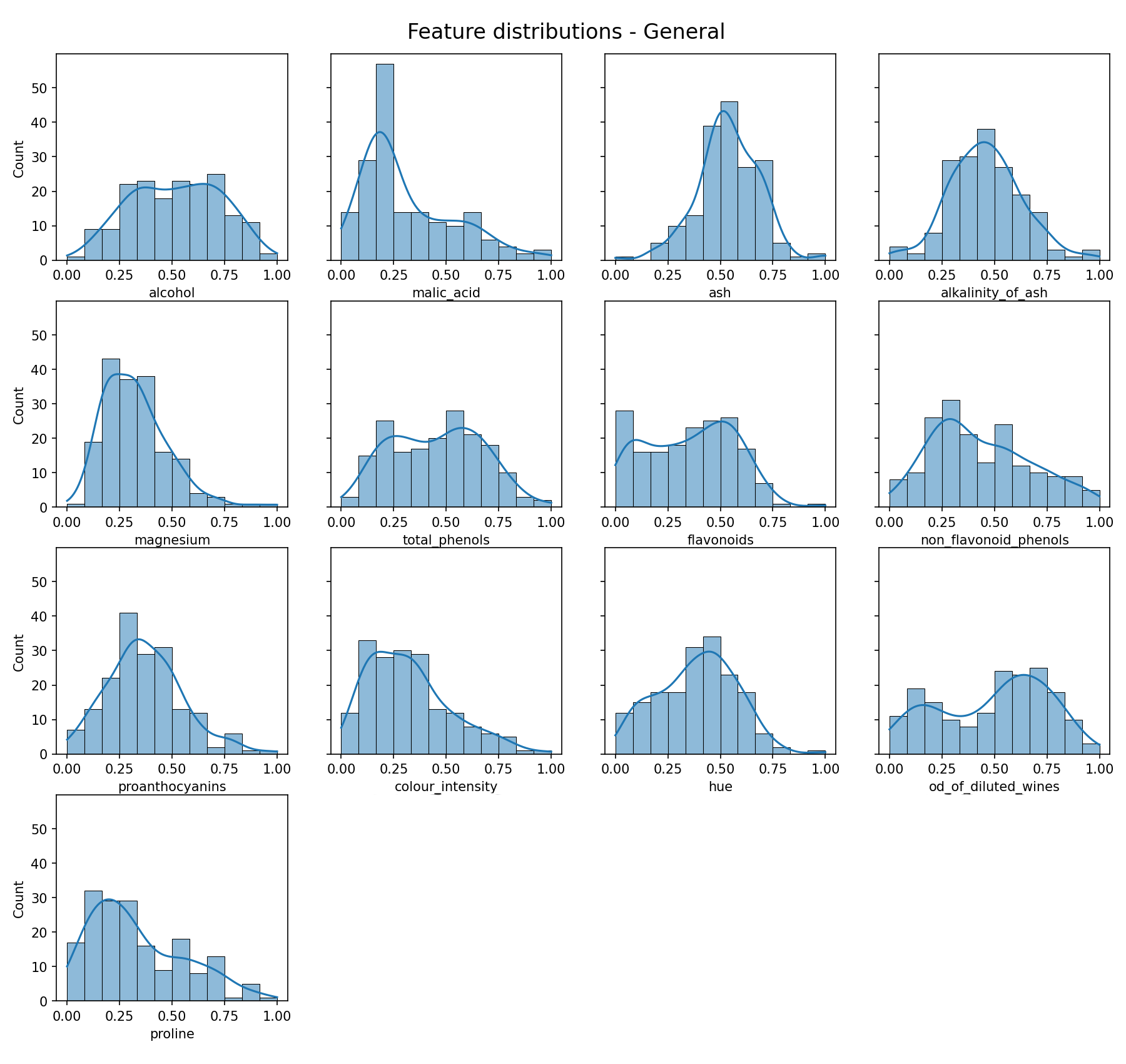
Feature data distribution — Image by author

Now some of those look quite Gaussian (e.g. alkalinity of ash), but the reality is most do not. Is this a problem? Well not necessarily, as what really exists in a lot of cases is a *mixture* of Gaussian distributions (or approximate Gaussian distributions).

The whole point of the Gaussian Mixture Model is that it can find and separate out the individual Gaussian distributions from a mixture of more than one Gaussian distribution.

In a real clustering problem you would not be able to achieve this next step, as you wouldn’t know the real clustering of the data. However, just for illustration purposes it is possible (as we know the labels) to plot each individual ‘real’ clusters distribution:

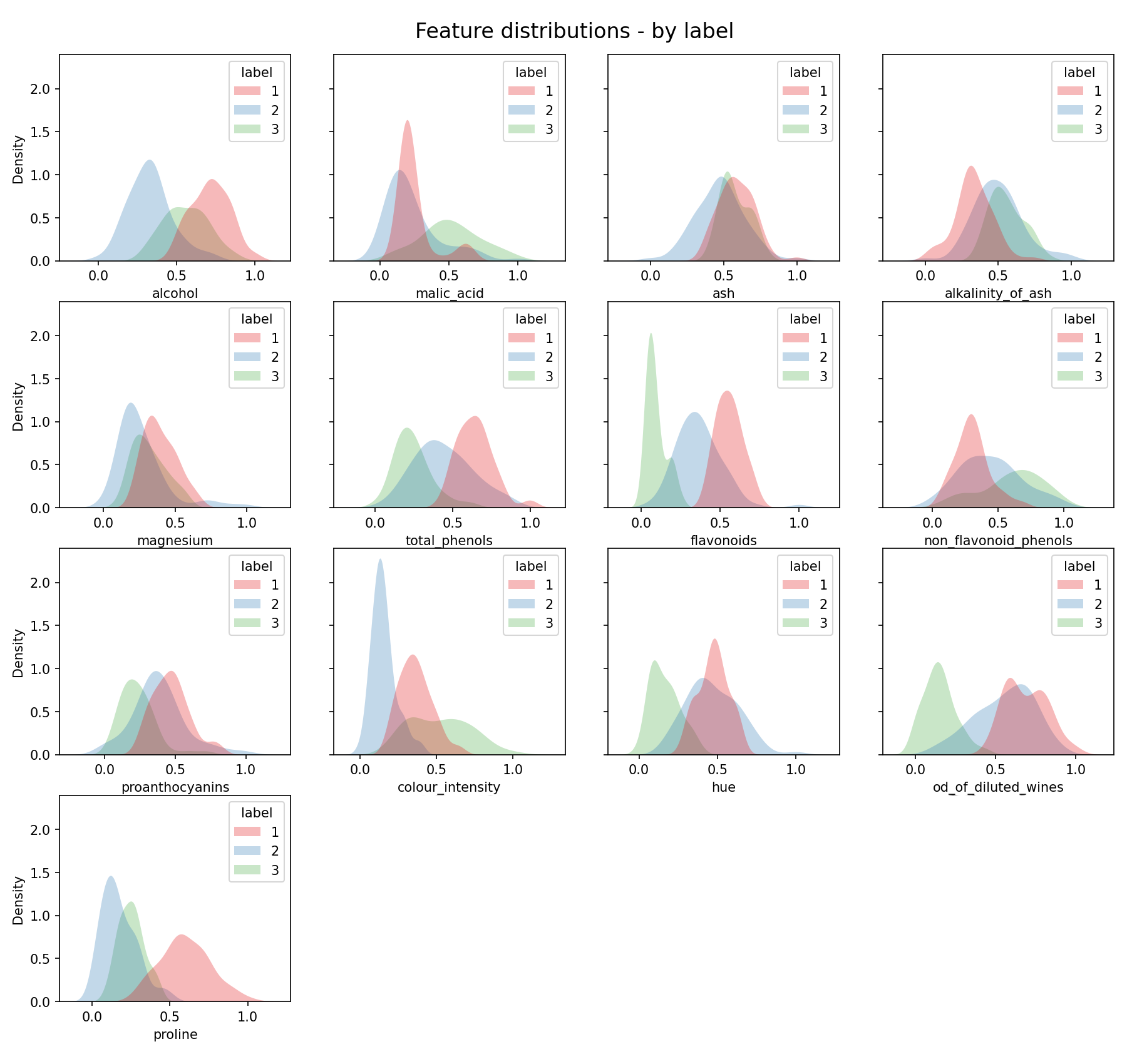
Feature data distribution by label — Image by author

As you can now see the real clusters are in most cases approximately Gaussian. This is not the case across the board, but it will never be the case with real data. As expected, due to the data being based on “natural” data we are indeed dealing with approximately Gaussian data.

This very basic investigation of the distribution of the raw data illustrates the importance of being aware of the type of data you are dealing with, and which tools would be best suited to the analysis. This is also a good case for the importance of domain experts, where appropriate.

Feature relations #

Finally, a few examples of how some of the variables are distributed in relation to each other (if you want a more comprehensive plot please take a look at the Jupyter notebook):

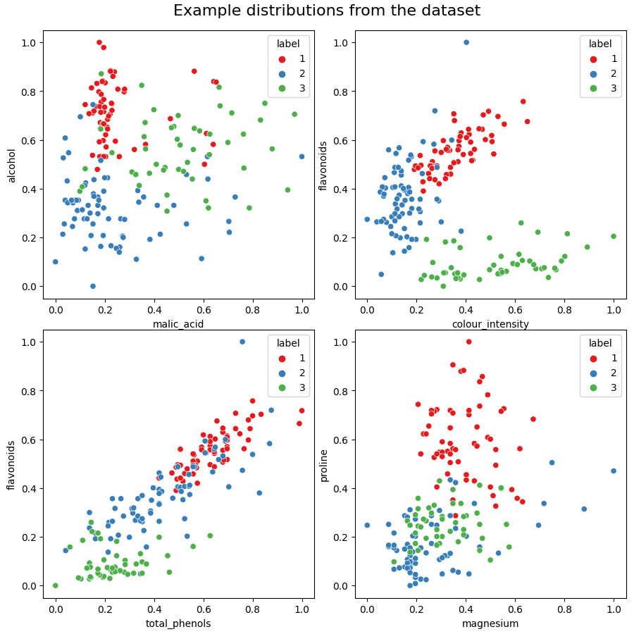
An example of the distribution of data between components — Image by author

As can be seen from the scatter plots above, some features show reasonable separation. However, there is also quite a lot of mixing with some features, and more so on the periphery of each cluster. The shape (circular, elongated etc.) also varies quite widely.

The Analysis #

Photo by Artem Podrez from Pexels

As mentioned earlier, there will be three different algorithms compared:

1. K-Means (the baseline)
2. Gaussian Mixture Model
3. Bayesian Gaussian Mixture Model

There will also be three phases to the exploration:

1. All of the raw data analysed at once
2. All of the data analysed after reducing complexity / features with a Principle Component Analysis (PCA)
3. An analysis using just two features (mainly to allow easier illustration than using the full dataset)

Analysis 1 — the full dataset #

To keep the comparison consistent, and reduce the complexity of this article I am going to skip a thorough investigation into how many components is the correct number.

However, just for completeness you should be aware that a crucial step in performing any clustering is gaining an understanding of the appropriate amount of clusters to use. Some common examples of how to achieve this are the elbow method, the Bayesian Information Criterion (BIC) and the Akaike information criterion. As an example here are the BIC and AIC for the whole raw dataset:

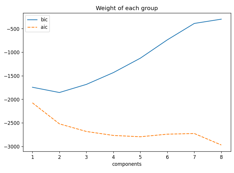
The BIC and AIC curves for this dataset — Image by Author

The BIC would suggest two components is appropriate, but I’m not going to go further into this result for now. However, it will come up in discussion later in the article.

Three clusters will be assumed from now on for consistency and ease of comparison.

Let’s get stuck in!

K-Means #

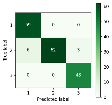
K-Means confustion matrix — Image by author

Well that is a fairly impressive result.

With all data taken together there is apparently very good separation between clusters 1 and 3. However, as cluster 2 generally sits between clusters 1 and 3 (refer back to the four example scatter plots in the previous section) it would appear that the points on the periphery of cluster 2 are being wrongly assigned to clusters 1 and 3 (i.e. the boundaries between those clusters are likely incorrectly defined).

Let’s see if this improves with a Gaussian Mixture Model.

Gaussian Mixture Model #

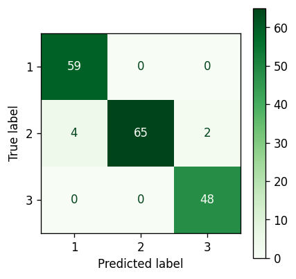
Gaussian Mixture Model confusion matrix — Image by author

An improvement. The Gaussian Mixture Model has managed to pick up three extra points and assign them correctly to cluster 2.

Although that doesn’t seem like a big deal, it is worth bearing in mind that the dataset is quite small, and using a more comprehensive dataset would likely yield a more impressive number of points.

Bayesian Gaussian Mixture Model #

Before producing the result, and as this is the main focus of the article, I think it is worth taking a little time to explain some of the relevant parameters that can be specified:

1. n_components — this is the number of clusters that you want the algorithm to consider. However, the algorithm may return, or prefer, less clusters than set here, which is one of the main advantages of this algorithm (we will see this in action soon)
2. covariance_type — there are four options here full, tied, diag and spherical. The most ‘accurate’ and typically preferred is full. This parameter essentially decides the limitation of the distribution fit shape, a great illustration is provided here.
3. weight_concentration_prior_type — this can either be dirichlet_process (infinite mixture model) or dirichlet_distribution (finite mixture model). In general, it is better to opt for the Dirichlet process as it is less sensitive to parameter changes, and does not tend to divide natural clusters into unnecessary sub-components as the Dirichlet distribution can sometimes do.
4. weight_concentration_prior — specifying a low value (e.g. 0.01) will cause the model to set a larger number of components to zero leaving just a few components remaining with significant value. High values (e.g. 100000) will tend to allow a larger number of components to remain active with relevant values i.e. less components will be set to zero.

As there are quite a lot of extra parameters it may be wise to perform cross validation analysis in some cases. For example, in this initial run covariance_type will be set to ‘diag’ rather than ‘full’ as the suggested cluster number is more convincing. I suspect in this specific case this is due to a combination of a smaller dataset, and a large number of features causing the ‘full’ covariance type to over-fit.

It is now possible to review what the algorithm has decided in terms of relevant clusters. This is possible by extracting the weights from the fitted model:

A bit more clearly in graph form:

Bayesian Gaussian Mixture Model group weights — Image by author

To be honest, not very convincing.

It is clear that there are three clusters ahead of the rest, but this is only intuitive because the answer is known. The truth is it is not very clear. So why is this?

The main reason is likely due to a combination of lack of data, and a high number of features (at least compared to the amount of data).

Lack of data will cause items such as outliers to have a much larger effect on the overall distribution, but also reduce the models ability to generate a distribution in the first place.

In the sections that follow we will look at a way to potentially combat this, and also at analysing a smaller selection of features to see what result we get in those circumstances.

For now, as we know the correct number of components is three we will push on.

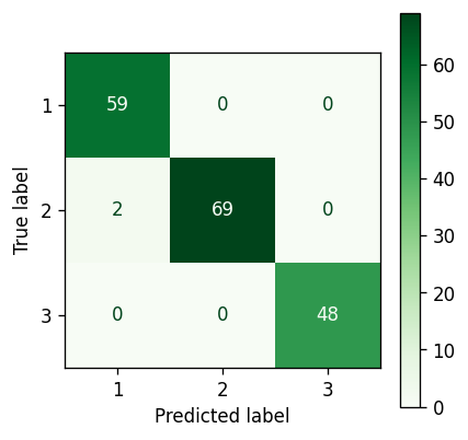
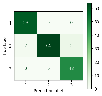
Bayesian Gaussian Mixture Model confusion matrix — Image by author

Almost perfect clustering. Only two points remain incorrectly assigned.

Let’s take a quick look at an overall comparison.

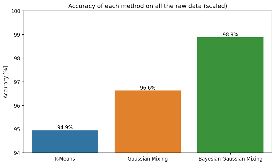
Accuracy comparison of the different clustering methods — Image by author

Discussion #

As can be seen from the accuracy results, there is a gradual improvement from one method to the next. This goes to show that understanding the structure of the underlying data is important, as it allows a more accurate representation of the patterns within the raw data, in our case Gaussian distributions.

Even within the realm of Gaussian Mixture Models, it is also clear (at least in this case) that the use of variational inference in the Bayesian Gaussian Mixture Model can yield more accurate results than expectation-maximisation.

All of this was expected, but it is interesting to see nonetheless.

Visualisation #

To give a general overview of what exactly the Gaussian algorithms are doing, I have plotted the feature “alcohol” against each of the other features, and also included the confidence ellipses of the Bayesian Gaussian Mixture Model on each plot for each of the three clusters.

Note: the algorithm used to draw the confidence ellipses is adapted from this algorithm provided in the scikit-learn documentation.

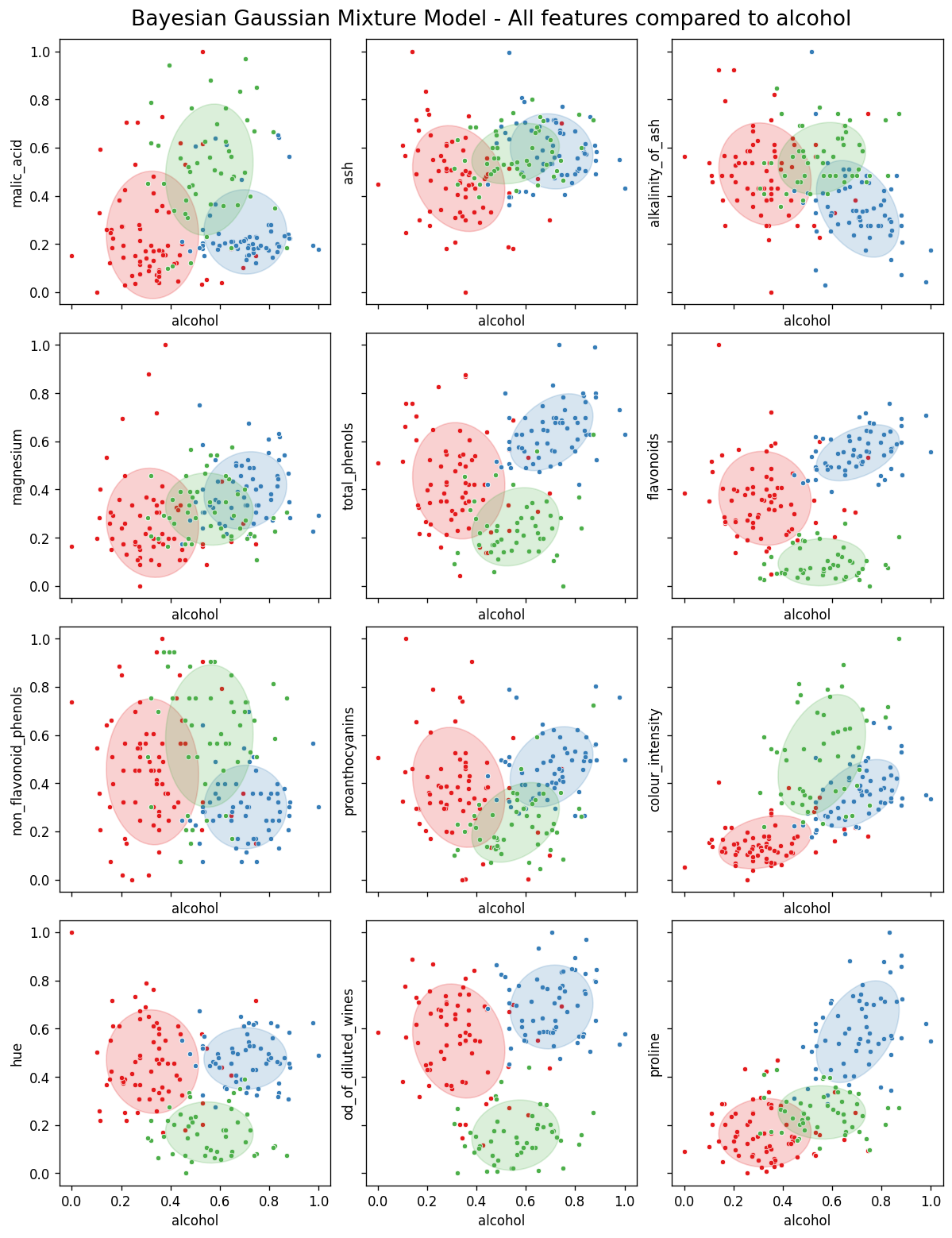
Bayesian Gaussian Mixture Model - Alcohol compared to all other features — Image by author

Although this is interesting to look at, and does do a good job of showing how the algorithm can account for the various shapes of the clusters (i.e. round, of more elongated ellipses) it doesn’t allow any sort of understanding as to what factors may have influenced the outcome.

This is mainly due to the fact that there are too many dimensions to deal with (i.e. too many features) in terms of representing the output as something interpretable.

Better visualisation and further investigation #

It would be interesting to visualise and compare the distributions produced by the various methods in a clear and concise way, so that it is possible to see exactly what is going on under the hood.

However, due to the large amount of features (and therefore dimensions) the model is processing, it is not possible to represent what is going on in a simple 2D graph, as has just been illustrated in the previous section.

With this in mind the aim of the next two sections of this article is to simplify the analysis by reducing the dimensions. The following two sections of this article will therefore look into:

1. the use of a two component Principle Component Analysis (PCA). This will allow all of the thirteen features to be distilled into two features, whilst keeping the *majority* of the important information embedded in the data.
2. specifically using only two features to run the analysis.

Both of these investigations will allow a direct visualisation of the clusters as there are only two components, and therefore it is then possible to plot them on a standard 2D graph.

Furthermore, these approaches will potentially make it easier to use the Bayesian Gaussian Mixture Model’s automatic cluster selection more effectively, as the amount of features in relation to the number of examples is more in balance.

Analysis 2 — Principle Component Analysis (PCA) #

By running a two component Principle Component Analysis (PCA) the 13 features can be compressed down to 2 components.

The main aims for this section are as follows:

1. Gain insights into the data distribution from the reduced complexity afforded by the PCA before analysis.
2. Review the automatic component selection generated by the Baysian Gaussian Mixture Model from the PCA dataset.
3. Run the Bayesian Gaussian Mixture Model on the two PCA components, and review the clustering result in 2D graph form.

The result of the PCA #

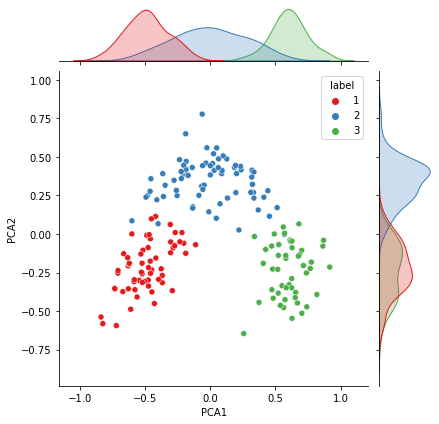
The two components of the PCA on all the data with distributions (colours are real label clusters) — Image by Author

The result of the PCA is interesting for quite a few reasons.

Firstly, the distribution of the primary PCA component (and to some degree the secondary PCA component) is very close to a Gaussian distribution for all three components. Mirroring what we have discovered from the data investigation earlier in the article.

Remembering for a second that the PCA is a distillation of all of the features, it is interesting to see that there is good separation between the three real clusters. This means there is a very good possibility that a clustering algorithm that targets the data well (regardless of the PCA) has the potential to achieve a good and accurate separation of the clusters.

However, the clusters are close enough, that if the clustering algorithm does not represent the distribution, or shape, of the clusters correctly, there is no guarantee that the boundary between the clusters will be found accurately.

For example, the distribution of cluster 1 is quite clearly elongated along the y-axis. Any algorithm would need to mimic this elongated shape to represent that particular cluster correctly.

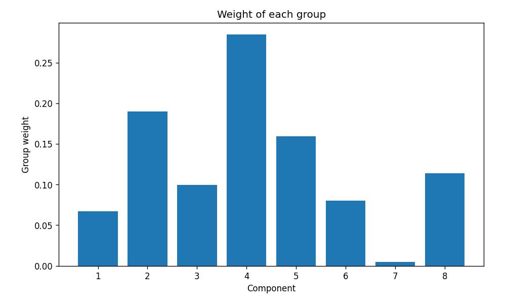
Automatic Clusters #

In the initial analysis the automatic estimation of the correct number of clusters was a little ambiguous. Now that the data complexity has been reduced let’s see if there is any improvement.

Again, the inputs request 8 components:

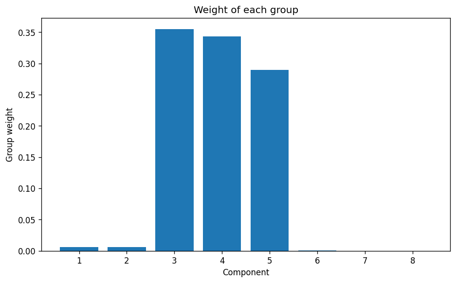
The weights of each of the 8 requested clusters — Image by Author

…and there we are. A very clear indication that even though the model was set up to consider up to 8 clusters, the algorithm clearly thinks that the actual appropriate number of clusters is 3. Which we of course know to be correct.

This goes some way to indicate that for the Bayesian Gaussian Mixture Model to work effectively, in terms of automatic cluster selection, it is necessary to consider whether the dataset is large enough to generate a reasonable and definitive result if the number of clusters is not already known.

The result #

For completeness let’s see how the clustering for the Bayesian Gaussian Mixture Model of the PCA went.

Bayesian Gaussian Mixture Model (PCA) confusion matrix — Image by author

A definite accuracy drop when compared to using the raw data. This is of course expected. By running a PCA we are definitely losing data, there is no avoiding that, and in this case it is enough to introduce an additional 5 misassigned data points.

Let’s look at this visually in a little more detail.

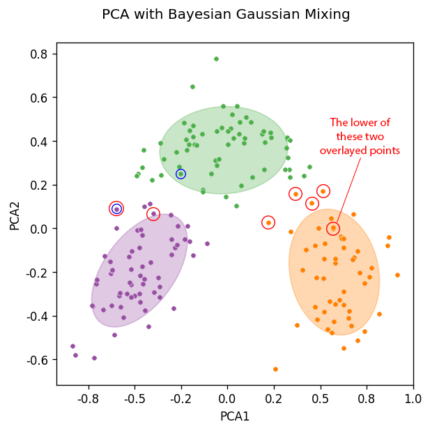
Bayesian Gaussian Mixing of a two component PCA (mismatched points ringed red) — Mismatched points from original analysis of all data ringed in blue — Image by Author

The graph above has a lot going on, so let’s break this down:

1. the coloured dots are the clusters that the PCA data was assigned to by the algorithm.
2. the large shaded ellipses are the confidence ellipses, which essentially state the shape of the underlying distribution generated by the algorithm (co-variances).
3. the red circles are the data points that have been misassigned by the Bayesian Gaussian Mixing Model from the PCA analysis.
4. the blue circles are the data points that were misassigned by the Bayesian Gaussian Mixing Model in the original analysis that used all of the raw data.

What is particularly interesting is that by running the PCA analysis, and likely due to the inherent loss of data, it forces some data points to be shifted well within the clusters / confidence ellipses that are generated (look at the orange point labelled with text, and dot circled blue within the green confidence ellipsoid).

In the case of the blue circled green point it helped, it is an improvement over the original ‘all raw data’ analysis. However, it is quite clear the orange point that is misassigned would never be correctly assigned, as it too well embedded within the orange cluster, when in fact it should be in the green cluster. However, the original analysis correctly assigned this data point to the green cluster.

PCA Summary #

In this particular case, it was useful with a smaller dataset to run a PCA to help the Bayesian Gaussian Mixture Model fix on an appropriate number of clusters. Even as an aid in getting a good visual grasp of how the dataset is distributed, it is potentially very useful.

However, it would not be an optimal solution to use the data generated by the PCA as a final input into the analysis. It is clear that the data shift / loss is sufficient enough as to potentially make some data points permanently wrongly assigned, and the overall accuracy is also reduced.

Analysis 3 — Fewer features #

To take a closer look at the differences between the three clustering algorithms two specific features will be extracted, and the clustering algorithms run on only those features.

The advantage of this in terms of reviewing the methods, is that it becomes possible to visualise what is going on a 2D-plane (i.e. a normal 2D graph).

An added bonus, is that the available data has much less information than the whole dataset. This both reduces the discrepancy between the small number of samples and the number of features, whilst also forcing the clustering algorithms to work much harder to achieve an appropriate fit due to the reduced information.

A closer look at the data #

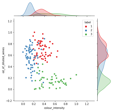
Colour intensity vs OD280/OD315 of diluted wines (raw data with labels) — Image by author

The reason for picking this pair (colour intensity and OD280/OD315 of diluted wines) is due to the challenges the dataset throws up for the different clustering algorithms.

As you can see there are two clusters that are fairly intermingled (1 & 2). In addition, clusters 2 & 3 have quite elongated distributions compared to cluster 1, which is more rounded, or circular.

In theory, the Gaussian mixing methods should fair quite a bit better than K-Means as they have the ability to accurately mould their distribution characteristics to the elongated distributions, whereas K-Means cannot, as it is limited to a circular representation.

Furthermore, from the KDE plots at each side of the graph it is possible to see that the data distribution is reasonably Gaussian as we have confirmed a few times before in this article.

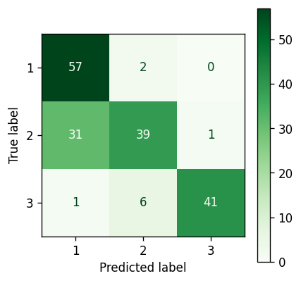
K-Means — Results #

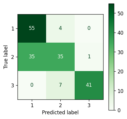
Confusion matrix for the K-Means - Reduced features — Image by author

Gaussian Mixture Model — Results #

Confusion matrix for the Gaussian Mixture Model — Reduced features — Image by author

Bayesian Gaussian Mixture Model — Component selection #

Before diving straight into the results, as the Bayesian Gaussian Mixture Model has the ability to auto-select the appropriate number of components we will again ‘request’ 8 components and see what the model suggests.

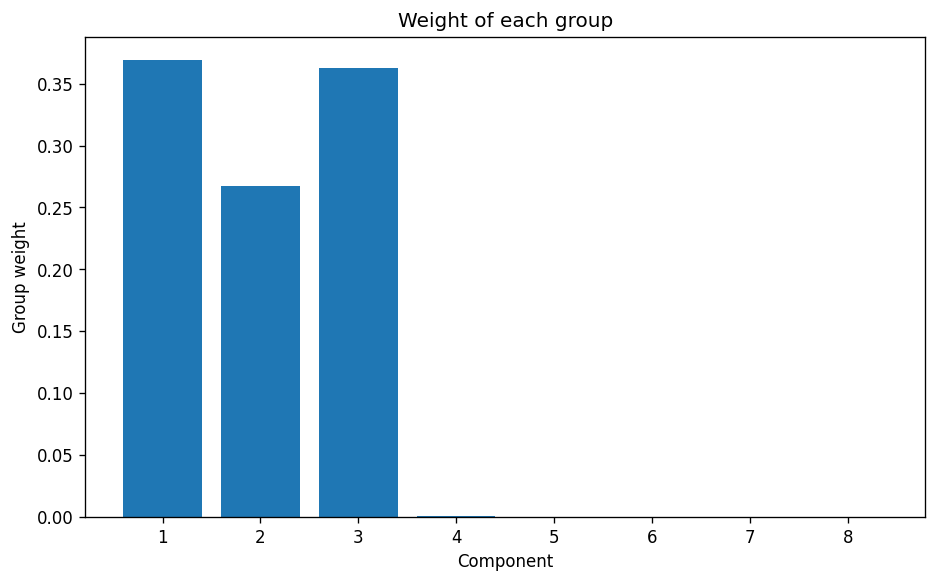
Component selection for the Bayesian Gaussian Mixture Model with two features only — Image by author

As previously seen with the reduced complexity of the PCA analysis, the model has found it much easier to distinguish the 3 clusters that are known to exist.

This would fairly conclusively confirm that:

1. it is necessary to have sufficient data samples to ensure that the model can stand a decent chance of offering the correct suggestion for number of clusters. This is likely due to the need to have enough data to properly represent the underlying distribution. In this case Gaussian.
2. a potential way to combat lack of samples is to in some way simplify or generalise the data to try and extract the appropriate number of clusters, and then revert to the full dataset for a final full clustering analysis

Bayesian Gaussian Mixture Model — Results #

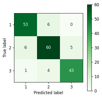
Confusion matrix for the Bayesian Gaussian Mixture Model — Reduced features — Image by author

Final results comparison #

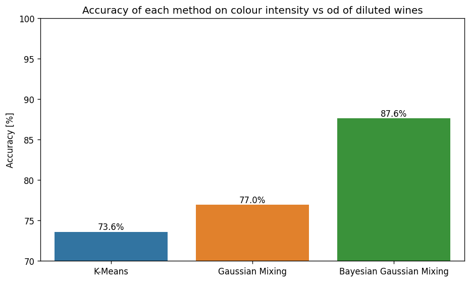
The accuracy of each clustering method for features colour intensity and OD280/OD315 of diluted wines — Image by author

As expected, the accuracy is a lot lower than when using the full dataset. However, regardless of this fact, there are some stark differences between the accuracy of the various methods.

Let’s dig a little deeper by comparing everything side-by-side.

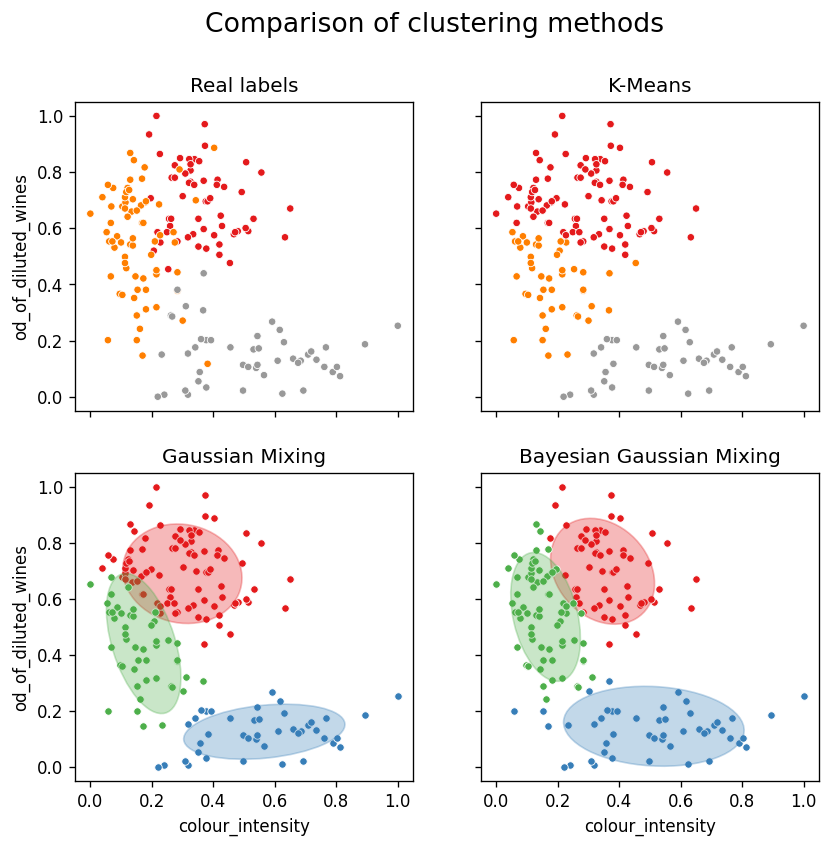
A comparison of the assignment of clusters for each of the three clustering methods — Cluster 1 (red) / Cluster 2 (orange/green) / Cluster 3 (grey/blue) — Image by author

The first thing to note is that the real labels show that there is a certain amount of fairly deep mixing / crossover between the clusters in some instances, so 100% accuracy is out of the question.

Reference for the following discussion:

• Cluster 1 — Red
• Cluster 2 — Orange/Green
• Cluster 3 — Grey/Blue

K-means #

K-means does a reasonable job of splitting out the clusters, but due to the fact that the distributions must ultimately be limited to a circular shape, there was never any hope of accurately capturing clusters 2 or 3 precisely.

However, as cluster 3 is quite well separated from the other two, the elongated shape is less of a hindrance. A circular representation of the lower cluster is actually sufficient, and gives a comparable representation to the Gaussian methods.

When considering clusters 1 and 2 the K-Means method fails to sufficiently represent the data. It has an inherent inability to properly represent the elliptical shape of cluster 2. This causes cluster 2 to be ‘squashed’ down in between clusters 1 and 3 as the real extension upwards cannot be sufficiently described by the K-Mean algorithm.

Gaussian Mixture Model #

The basic Gaussian Mixture Model is only a slight improvement in this case.

As discussed in the previous section for K-Means, even though the distribution of cluster 3 is better suited to an elliptical rather than circular distribution, it is of no advantage in this particular scenario.

However, when looking at the representation of cluster 1 and 2, which are significantly more intertwined, the ability of the Gaussian Mixture Model to represent the underlying elliptical distribution (i.e. better capturing the underlying tails of the Gaussian distribution) of cluster 2 more accurately, results in a slight increase in accuracy.

Bayesian Gaussian Mixture Model #

For a start, the more than 10% improvement in accuracy of the Bayesian Gaussian Mixture Model compared to the other methods is certainly impressive as a lone statistic.

On review of the confidence ellipsoids it becomes clear why this is the case. Cluster 2 has been represented both in terms of shape, tilt and size just about as perfectly as it could be. This has allowed for a very accurate representation of the real clusters.

Although the exact reasons for this will always be slightly opaque, it is most definitely down to the differences between the expectation-maximisation algorithm used by the standard Gaussian Mixture Model, and the variational inference used by the Bayesian Gaussian Mixture Model.

As discussed earlier in the article, the main differences are:

• the in built regularisation
• less tendency for variational inference to generate ‘marginally correct’ solutions to the problem

Conclusion #

It is quite clear that the use of Gaussian Mixture Models can help to elevate the accuracy of the clustering of data that is likely to have Gaussian distributions as it’s underpinning.

This is particularly relevant and useful for natural processes, including human processes, which make this analytical approach relevant to a large number of industries, across a wide variety of fields.

Furthermore, the introduction of variational inference in the Bayesian Gaussian Mixture Model can, with very little difference in overhead, return further improved accuracy in clustering. There is even the, not so insignificant bonus, of the algorithm having the ability to suggest the appropriate amount of clusters for the underlying data.

I hope this article has provided you with a decent insight into what Gaussian Mixing Models and Bayesian Gaussian Mixture Models are, and whether they may help with data you are working with.

They really are a powerful tool if used appropriately.

References #

[1] Riccardo Leardi, Wine (1991), UC Irvine Machine Learning Repository, License: CC BY 4.0

🙏🙏🙏

Since you've made it this far, sharing this article on your favorite social media network would be highly appreciated. For feedback, please ping me on Twitter.

...or if you want fuel my next article, you could always:

Published 15 Feb 2023